The dot product

$\newenvironment {prompt}{}{} \newcommand {\ungraded }[0]{} \newcommand {\todo }[0]{} \newcommand {\oiint }[0]{{\large \bigcirc }\kern -1.56em\iint } \newcommand {\mooculus }[0]{\textsf {\textbf {MOOC}\textnormal {\textsf {ULUS}}}} \newcommand {\npnoround }[0]{\nprounddigits {-1}} \newcommand {\npnoroundexp }[0]{\nproundexpdigits {-1}} \newcommand {\npunitcommand }[1]{\ensuremath {\mathrm {#1}}} \newcommand {\RR }[0]{\mathbb R} \newcommand {\R }[0]{\mathbb R} \newcommand {\N }[0]{\mathbb N} \newcommand {\Z }[0]{\mathbb Z} \newcommand {\sagemath }[0]{\textsf {SageMath}} \newcommand {\d }[0]{\,d} \newcommand {\l }[0]{\ell } \newcommand {\ddx }[0]{\frac {d}{\d x}} \newcommand {\zeroOverZero }[0]{\ensuremath {\boldsymbol {\tfrac {0}{0}}}} \newcommand {\inftyOverInfty }[0]{\ensuremath {\boldsymbol {\tfrac {\infty }{\infty }}}} \newcommand {\zeroOverInfty }[0]{\ensuremath {\boldsymbol {\tfrac {0}{\infty }}}} \newcommand {\zeroTimesInfty }[0]{\ensuremath {\small \boldsymbol {0\cdot \infty }}} \newcommand {\inftyMinusInfty }[0]{\ensuremath {\small \boldsymbol {\infty -\infty }}} \newcommand {\oneToInfty }[0]{\ensuremath {\boldsymbol {1^\infty }}} \newcommand {\zeroToZero }[0]{\ensuremath {\boldsymbol {0^0}}} \newcommand {\inftyToZero }[0]{\ensuremath {\boldsymbol {\infty ^0}}} \newcommand {\numOverZero }[0]{\ensuremath {\boldsymbol {\tfrac {\#}{0}}}} \newcommand {\dfn }[0]{\textbf } \newcommand {\unit }[0]{\mathop {}\!\mathrm } \newcommand {\eval }[1]{\bigg [ #1 \bigg ]} \newcommand {\seq }[1]{\left ( #1 \right )} \newcommand {\epsilon }[0]{\varepsilon } \newcommand {\phi }[0]{\varphi } \newcommand {\iff }[0]{\Leftrightarrow } \DeclareMathOperator {\arccot }{arccot} \DeclareMathOperator {\arcsec }{arcsec} \DeclareMathOperator {\arccsc }{arccsc} \DeclareMathOperator {\si }{Si} \DeclareMathOperator {\scal }{scal} \DeclareMathOperator {\sign }{sign} \newcommand {\arrowvec }[1]{{\overset {\rightharpoonup }{#1}}} \newcommand {\vec }[1]{{\overset {\boldsymbol {\rightharpoonup }}{\mathbf {#1}}}\hspace {0in}} \newcommand {\point }[1]{\left (#1\right )} \newcommand {\pt }[1]{\mathbf {#1}} \newcommand {\Lim }[2]{\lim _{\point {#1} \to \point {#2}}} \DeclareMathOperator {\proj }{\mathbf {proj}} \newcommand {\veci }[0]{{\boldsymbol {\hat {\imath }}}} \newcommand {\vecj }[0]{{\boldsymbol {\hat {\jmath }}}} \newcommand {\veck }[0]{{\boldsymbol {\hat {k}}}} \newcommand {\vecl }[0]{\vec {\boldsymbol {\l }}} \newcommand {\uvec }[1]{\mathbf {\hat {#1}}} \newcommand {\utan }[0]{\mathbf {\hat {t}}} \newcommand {\unormal }[0]{\mathbf {\hat {n}}} \newcommand {\ubinormal }[0]{\mathbf {\hat {b}}} \newcommand {\dotp }[0]{\bullet } \newcommand {\cross }[0]{\boldsymbol \times } \newcommand {\grad }[0]{\boldsymbol \nabla } \newcommand {\divergence }[0]{\grad \dotp } \newcommand {\curl }[0]{\grad \cross } \newcommand {\lto }[0]{\mathop {\longrightarrow \,}\limits } \newcommand {\bar }[0]{\overline } \newcommand {\surfaceColor }[0]{violet} \newcommand {\surfaceColorTwo }[0]{redyellow} \newcommand {\sliceColor }[0]{greenyellow} \newcommand {\vector }[1]{\left \langle #1\right \rangle } \newcommand {\sectionOutcomes }[0]{} \newcommand {\HyperFirstAtBeginDocument }[0]{\AtBeginDocument }$

The dot product measures how aligned two vectors are with each other.

The definition of the dot product

We have already seen how to add vectors and how to multiply vectors by scalars.

We have not yet defined how to multiply a vector by a vector. You might think it is reasonable to define $\begin {bmatrix} a_1\\ a_2\\ \vdots \\ a_n \end {bmatrix} \cdot \begin {bmatrix} b_1\\ b_2\\ \vdots \\ b_n \end {bmatrix} = \begin {bmatrix} a_1b_1\\ a_2b_2\\ \vdots \\ a_nb_n \end {bmatrix}$ but this operation is not especially useful, and will never be utilized in this course.

In this section we will define a way to “multiply” two vectors called the dot product. The dot product measures how “aligned” two vectors are with each other.

The dot product of two vectors is given by the following. $\begin{align*} \begin{bmatrix} a_1\\ a_2\\ \vdots\\ a_n \end{bmatrix} \dotp \begin{bmatrix} b_1\\ b_2\\ \vdots\\ b_n \end{bmatrix} &= \sum_{i=1}^n a_ib_i\\ &= a_1b_1 + a_2b_2 +\dots+a_nb_n \end{align*}$

The first thing you should notice about the the dot product is that $\mathbf {vector}\dotp \mathbf {vector} = \mathbf {number}.$

Compute. $\vector {1,2,3}\dotp \vector {4,5,6} \begin {prompt} = \answer {32} \end {prompt}$

Compute. $\vector {1,1,-1}\dotp \vector {1,1,2} \begin {prompt} = \answer {0} \end {prompt}$

Let $\vec {u},\vec {v},\vec {w}$ be nonzero vectors in $\R ^3$ . Which of the following expressions make sense?

$(\vec {w} \dotp \vec {u} ) \vec {u}$ $5(\vec {u} +\vec {w}) \dotp {\vec {u}}$ $\vec {w} / \vec {u}$ $\vector {2,3} \dotp \vector {4,2} + 7$ $\vec {w} / ( \vec {u} \dotp \vec {u})$ $\vector {1,3} \dotp \vector {-1,2,5}$ $\vec {u}\dotp \vec {v}+\vec {w}$

Think about which terms/factors are vectors and which terms/factors are scalars.

Which of the following are vectors?

$(\vec {w} \dotp \vec {u} ) \vec {u}$ $5(\vec {u} +\vec {w}) \dotp {\vec {u}}$ $\vector {2,3} \dotp \vector {4,2} + 7$ $\vec {w} / ( \vec {u} \dotp \vec {u})$

The dot product allows us to write some complicated formulas more simply.

The magnitude of vector $\vec {v}$ is given by $|\vec {v}|=\sqrt {\vec {v}\dotp \vec {v}}$

We already know that if $\vec {v} = \vector {v_1,v_2,\dots ,v_n}$ , then $|\vec {v}| = \sqrt {v_1^2+v_2^2+v_3^2+\dots +v_n^2}$ but $\vec {v} \dotp \vec {v} = v_1^2+v_2^2+v_3^2+\dots +v_n^2,$ so $|\vec {v}|=\sqrt {\vec {v}\dotp \vec {v}}.$

Compute the magnitude of the vector $\vec {v} = \vector {1,2,3,4}$ . $|\vec {v}| = \answer {\sqrt {30}}$

The geometry of the dot product

Let’s see if we can figure out what the dot product tells us geometrically. As an appetizer, we give the next theorem: the Law of Cosines.

Law of Cosines Given a triangle with sides of length $a$ , $b$ , and $c$ , and with $0\le \theta \le \pi$ being the measure of the angle between the sides of length $a$ and $b$ ,

we have $c^2 = a^2+b^2-2ab\cos (\theta ).$

When $\theta = \pi /2$ what does the law of cosines say?

It is the Pythagorean theorem. It is the law of sines. It is undefined.

We can rephrase the Law of Cosines in the language of vectors. The vectors $\vec {v}$ , $\vec {w}$ , and $\vec {v} - \vec {w}$ form a triangle

so if $\theta$ is the angle between $\vec {v}$ and $\vec {w}$ we must have $|\vec {v} - \vec {w}|^2=|\vec {v}|^2+|\vec {w}|^2-2|\vec {w}||\vec {v}|\cos (\theta ).$

Geometric Interpretation of the Dot Product For any two vectors $\vec {v}$ and $\vec {w}$ , $\vec {v} \dotp \vec {w} = |\vec {v}||\vec {w}|\cos (\theta )$ where $0\le \theta \le \pi$ is the angle between $\vec {v}$ and $\vec {w}$ .

First note that $|\vec {v} - \vec {w}|^2 = (\vec {v} - \vec {w})\dotp (\vec {v} - \vec {w})$ Now use the law of cosines to write $\begin{align*} |\vec{v} - \vec{w}|^2&=|\vec{v}|^2+|\vec{w}|^2-2|\vec{v}||\vec{w}|\cos(\theta)\\ (\vec{v} - \vec{w})\dotp(\vec{v} - \vec{w}) &=|\vec{v}|^2+|\vec{w}|^2-2|\vec{v}||\vec{w}|\cos(\theta)\\ \vec{v}\dotp\vec{v} -2\vec{v}\dotp\vec{w}+\vec{w}\dotp\vec{w}&=|\vec{v}|^2+|\vec{w}|^2-2|\vec{v}||\vec{w}|\cos(\theta)\\ |\vec{v}|^2+|\vec{w}|^2 -2\vec{v}\dotp\vec{w} &=|\vec{v}|^2+|\vec{w}|^2-2|\vec{v}||\vec{w}|\cos(\theta)\\ \vec{v} \dotp \vec{w} &= |\vec{v}||\vec{w}|\cos(\theta). \end{align*}$

The theorem above tells us some interesting things about the angle between two (nonzero) vectors.

If $\vec {v}$ and $\vec {w}$ are two nonzero vectors, and $\theta$ is the angle between them, $\vec {v}\dotp \vec {w} = 0 \text { if and only if } \theta = \frac {\pi }{2}.$

We have a special buzz-word for when the dot product is zero.

Two vectors are called orthogonal if the the dot product of these vectors is zero.

Note: Geometrically, this means that the angle between two nonzero vectors is $\pi /2$ or $90^\circ$ . This also means that the zero vector is orthogonal to all vectors.

From this we see that the dot product of two vectors is zero if those vectors are orthogonal. Moreover, if the dot product is not zero, using the formula $\vec {v} \dotp \vec {w} = |\vec {v}||\vec {w}|\cos (\theta )$ allows us to compute the angle between these vectors via $\theta = \arccos \left (\frac {\vec {v} \dotp \vec {w} }{|\vec {v}|\cdot |\vec {w}|}\right ),$ where $0\le \theta \le \pi$ .

Find the angle between the vectors. $\begin{align*} \vec{v} &= 2\veci+3\vecj+6\veck\\ \vec{w} &= 1\veci+2\vecj+2\veck \end{align*}$ $\theta = \answer { \arccos \left (\frac {20}{21}\right )}$

Think about how hard this question would have been before you read this section!

Find all unit vectors orthogonal to both vectors $\vec {v}$ and $\vec {w}$ , given by $\begin{align*} \vec{v} &= \veci + \vecj\\ \vec{w} &= \veci + \veck . \end{align*}$ Write your vectors in the order of increasing $x$ -components. $\vector {\answer {-1/\sqrt {3}},\answer {1/\sqrt {3}},\answer {1/\sqrt {3}}}\quad \text {and}\quad \vector {\answer {1/\sqrt {3}},\answer {-1/\sqrt {3}},\answer {-1/\sqrt {3}}}$

Projections and components

Projections

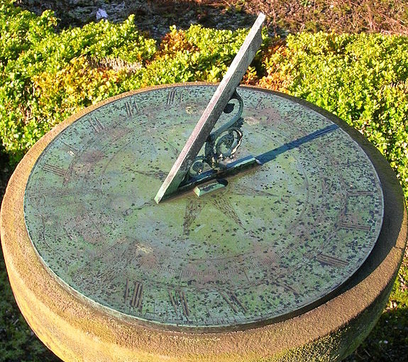
One of the major uses of the dot product is to let us project one vector in the direction of another. Conceptually, we are looking at the “shadow” of one vector projected onto another, sort of like in the case of a sundial.

In essence we imagine the “sun” directly over a vector, casting a shadow onto another vector.

While this is good starting point for understanding orthogonal projections, now we need the definition.

The orthogonal projection of vector $\vec {v}$ in the direction of vector $\vec {w}$ is a new vector denoted $\proj _\vec {w}(\vec {v})$

that lies on the line containing $\vec {w}$ , with the vector $\proj _\vec {w}(\vec {v}) - \vec {v}$ perpendicular to $\vec {w}$ . Below we see vectors $\vec {v}$ and $\vec {w}$ along with $\proj _{\vec {w}}(\vec {v})$ . Move the tips of vectors $\vec {v}$ and $\vec {w}$ to help you understand $\proj _{\vec {w}}(\vec {v})$ .

Consider the vector $\vec {v}=\vector {3,2,1}$ and the vector $\veci = \vector {1,0,0}$ . Compute $\proj _\veci (\vec {v})$ .

Draw a picture.

$\proj _\veci (\vec {v}) = \vector {\answer {3},\answer {0},\answer {0}}$

Let $\vec {v} = \vector {1,1}$ and $\vec {w}=\vector {-1,1}$ . Compute $\proj _\vec {w}(\vec {v})$ .

Draw a picture.

$\proj _\vec {w}(\vec {v}) = \vector {\answer {0},\answer {0}}$

To compute the projection of one vector along another, we use the dot product.

Given two vectors $\vec {v}$ and $\vec {w}$ $\proj _\vec {w}(\vec {v}) =\left (\frac {\vec {v} \dotp \vec {w}}{|\vec {w}|^2}\right ) \vec {w} =\left (\frac {\vec {v} \dotp \vec {w}}{\vec {w}\dotp \vec {w}}\right ) \vec {w}.$

First, note that the direction of $\proj _\vec {w}(\vec {v})$ is given by $\frac {\vec {w}}{|\vec {w}|}$ and the magnitude of $\proj _\vec {w}(\vec {v})$ is given by $|\proj _{\vec {w}}(\vec {v})| = |\vec {v}|\cdot \left | \answer [given]{\cos (\theta )}\right |.$

Now $\proj _\vec {w}(\vec {v}) = \mathrm {direction}\cdot \mathrm {magnitude},$ where $\mathrm {direction} = \pm \frac {\vec {w}}{|\vec {w}|}$ has a positive sign if $0<\theta < \pi /2$ , and a negative sign if $\pi /2< \theta < \pi$ . Also, $\mathrm {magnitude} = |\vec {v}|\cdot \left |\answer [given]{\cos (\theta )}\right |.$ Multiplying direction and magnitude we find the following. $\begin{align*} &= \frac{\vec{w}}{|\vec{w}|^2}\cdot |\vec{w}|\cdot |\vec{v}|\cdot\answer[given]{\cos(\theta)}\\ &= \left(\frac{\vec{v} \dotp \vec{w}}{|\vec{w}|^2}\right) \vec{w}\\ &=\left(\frac{\vec{v} \dotp \vec{w}}{\vec{w}\dotp \vec{w}}\right) \vec{w}. \end{align*}$ Notice that the sign of the direction is the sign of cosine, so we simply remove the absolute value from the cosine.

Find the projection of the vector $\vec {v} = \vector {2,3,1}$ in the direction of the vector $\vec {w} = \vector {3,-1,1}$ . $\proj _\vec {w}(\vec {v}) = \vector {\answer {\frac {12}{11}},\answer {\frac {-4}{11}},\answer {\frac {4}{11}}}$

Let $\vec {v}$ and $\vec {w}$ be nonzero vectors in $\R ^2$ . Let $k\ge 1$ . Select all statements that must be true.

$\proj _{\vec {w}}(\vec {v})=\proj _{\vec {v}}(\vec {w})$ $|\proj _{\vec {w}}(\vec {v})|\le |\vec {v}|$ $|\proj _{\vec {w}}(\vec {v})|\le |\vec {w}|$ $|\proj _{\vec {w}}(\vec {v})|\le |\proj _{\vec {w}}(k\cdot \vec {v})|$ $|\proj _{\vec {w}}(k\cdot \vec {v})|\le |\proj _{\vec {w}}(\vec {v})|$ $|\proj _{\vec {w}}(\vec {v})|\le |\proj _{k\cdot \vec {w}}(\vec {v})|$ $|\proj _{k\cdot \vec {w}}(\vec {v})|\le |\proj _{\vec {w}}(\vec {v})|$

Components

Scalar components compute “how much” of a vector is pointing in a particular direction.

Let $\vec {v}$ and $\vec {w}$ be vectors and let $0\le \theta \le \pi$ be the angle between them. The scalar component in the direction of $\vec {w}$ of vector $\vec {v}$ is denoted $\scal _\vec {w}(\vec {v})= \begin {cases} |\proj _\vec {w}(\vec {v})| &\text {when $0\le \theta \le \pi /2$}\\ -|\proj _\vec {w}(\vec {v})| &\text {when $\pi /2<\theta \le \pi $.} \end {cases}$

Let $\vec {v} = \vector {3,-2,1}$ . Compute $\scal _\veci (\vec {v})$ . $\scal _\veci (\vec {v}) = \answer {3}$

Compute $\scal _\vecj (\vec {v})$ . $\scal _\vecj (\vec {v}) = \answer {-2}$

Compute $\scal _\veck (\vec {v})$ . $\scal _\veck (\vec {v}) = \answer {1}$

To compute the scalar component of a vector in the direction of another, you use the dot product.

Given two vectors, $\vec {v}$ and $\vec {w}$ , $\scal _\vec {w}(\vec {v}) =\frac {\vec {v} \dotp \vec {w}}{|\vec {w}|}.$

Let $\vec {v}$ and $\vec {w}$ be nonzero vectors and let $\theta$ be the angle between them. Which of the following are true?

$|\proj _\vec {w}(\vec {v})| = \scal _{\vec {w}}(\vec {v})$ $|\proj _\vec {w}(\vec {v})| = |\scal _{\vec {w}}(\vec {v})|$ $\proj _\vec {w}(\vec {v}) =|\vec {v}|\cos (\theta )\left (\frac {\vec {w}}{|\vec {w}|}\right )$ $\scal _\vec {w}(\vec {v}) = |\vec {v}|\cos (\theta )$

Orthogonal decomposition

Given any vector $\vec {v}$ in $\R ^2$ , we can always write it as $\vec {v} = a\veci + b\vecj$ for some real numbers $a$ and $b$ . Here we’ve broken $\vec {v}$ into the sum of two orthogonal vectors — in particular, vectors parallel to $\veci$ and $\vecj$ . In fact, given a vector $\vec {v}$ and another vector $\vec {w}$ you can always break $\vec {v}$ into a sum of two vectors, one of which is parallel to $\vec {w}$ and another that is perpendicular to $\vec {w}$ . Such a sum is called an orthogonal decomposition. Move the point around to see various orthogonal decompositions of vector $\vec {v}$ .

Let $\vec v$ and $\vec w$ be vectors. The orthogonal decomposition of $\vec v$ in terms of $\vec {w}$ is the sum $\vec v = \underbrace {\proj _{\vec {w}}(\vec {v})}_{\parallel \vec w} + (\underbrace {\vec v-\proj _{\vec {w}}(\vec {v})}_{\perp \vec w}),$ where $\vec {x} \parallel \vec {y}$ means that “ $\vec {x}$ is parallel to $\vec {y}$ ” and $\vec {x} \perp \vec {y}$ means that “ $\vec {x}$ is perpendicular to $\vec {y}$ ”.

Let $\vec u = \vector {-2,1}$ and $\vec v = \vector {3,1}$ . What is the orthogonal decomposition of $\vec {u}$ in terms of $\vec {v}$ ? $\vec u= \underbrace {\vector {\answer {-1.5},\answer {-0.5}}}_{\parallel \vec v} + \underbrace {\vector {\answer {-0.5},\answer {1.5}}}_{\perp \vec v}$

Let $\vec w =\vector {2,1,3}$ and $\vec x =\vector { 1,1,1}$ . What is the orthogonal decomposition of $\vec {w}$ in terms of $\vec {x}$ ? $\vec w = \underbrace {\vector {\answer {2},\answer {2},\answer {2}}}_{\parallel \vec x} + \underbrace {\vector { \answer {0},\answer {-1},\answer {1}}}_{\perp \vec x}$

Now we give an example where this decomposition is useful.

Consider a box weighing $50\unit {lb}$ resting on a ramp that rises $5\unit {ft}$ over a span of $20\unit {ft}$ .

We know that the force of gravity is pointing straight down, but from experience, we know this exerts some sort of diagonal force on the box, too (things slide down ramps). This diagonal force will be described by the orthogonal decomposition of $\vec {g} = \vector {0,-50}$ in terms of $\vec {r}$ . Find this orthogonal decomposition.

To find the force of gravity in the direction of the ramp, we compute $\proj _\vec {r}(\vec g)$ . $\begin{align*} \proj_\vec{r}(\vec{g}) &= \left(\frac{\vec{g}\dotp\vec{r}}{\vec{r}\dotp\vec{r}}\right)\vec r\\ &= \answer[given]{\frac{-250}{425}}\vector{20,5}\\ &= \vector{\answer[given]{\frac{-200}{17}},\answer[given]{\frac{-50}{17}}} \end{align*}$ To find the component $\vec z$ of gravity orthogonal to the ramp, write with me. $\begin{align*} \vec z &= \vec g - \proj_\vec{r}(\vec{g}) \\ &= \vector{\answer[given]{\frac{200}{17}},\answer[given]{\frac{-800}{17}}} \end{align*}$

The algebra of the dot product

We summarize the arithmetic and algebraic properties of the dot product below.

The following are true for all scalars $s$ and vectors $\vec {u}$ , $\vec {v}$ , and $\vec {w}$ in $\R ^n$ .

Commutativity:: $\vec {v} \dotp \vec {w} = \vec {w} \dotp \vec {v}$
Linear in first argument:: $(\vec {u}+\vec {v})\dotp \vec {w} = \vec {u}\dotp \vec {w} + \vec {v}\dotp \vec {w}$ and $(s\vec {v})\dotp \vec {w} = s(\vec {v} \dotp \vec {w})$
Linear in second argument:: $\vec {u} \dotp (\vec {v}+\vec {w}) = \vec {u}\dotp \vec {v}+ \vec {u}\dotp \vec {w}$ and $\vec {v} \dotp (s\vec {w}) = s(\vec {v} \dotp \vec {w})$
Relation to magnitude:: $\vec {v} \dotp \vec {v} = |\vec {v}|^2$
Relation to orthogonality:: If $\vec {v}$ is orthogonal to $\vec {w}$ then $\vec {v} \dotp \vec {w} = 0$ .

Instead of defining the dot product by a formula, we could have defined it by the properties above! While this is common practice in mathematics, the process is a bit abstract and is perhaps beyond the scope of this course. Nevertheless, we know that you are an intrepid young mathematician, and we will not hold back. We will now show that there is only one formula which gives us all of these properties, and it will be our formula for the dot product.

The dot product is given by the following formula. $\begin{align*} \begin{bmatrix} a_1\\ a_2\\ \vdots\\ a_n \end{bmatrix} \dotp \begin{bmatrix} b_1\\ b_2\\ \vdots\\ b_n \end{bmatrix} &= \sum_{i=1}^n a_ib_i\\ &= a_1b_1 + a_2b_2 +\dots+a_nb_n \end{align*}$

Let $\uvec {e}_j = \vector {0,0,0,\dots ,1,\dots ,0}$ be the vector whose $j$ th coordinate is $1$ , with all other coordinates being $0$ . Then, we can write $\vector {a_1,a_2, \dots ,a_n} = \sum _{i=1}^n a_i \uvec {e}_i$ and $\vector {b_1,b_2, \dots ,b_n} = \sum _{i=1}^n b_j \uvec {e}_j.$ We now compute $\begin {bmatrix} a_1\\ a_2\\ \vdots \\ a_n \end {bmatrix} \dotp \begin {bmatrix} b_1\\ b_2\\ \vdots \\ b_n \end {bmatrix} = \left (\sum _{i=1}^n a_i \uvec {e}_i\right ) \dotp \left (\sum _{j=1}^n b_j \uvec {e}_j\right ).$ By the linearity properties of the dot product, the above is equal to $\sum _{i,j =1}^n a_ib_j(\uvec {e}_i \dotp \uvec {e}_j).$ Finally, since $\uvec {e}_i \dotp \uvec {e}_j = 1$ if $i=j$ (because they are parallel in this case) and $0$ otherwise (because then they are orthogonal). So, our expression becomes $\begin{align*} &\sum_{i=1}^n a_ib_i \\ &=a_1b_1 + a_2b_2 +\dots+a_nb_n. \end{align*}$