Lagrange multipliers

$\newenvironment {prompt}{}{} \newcommand {\ungraded }[0]{} \newcommand {\todo }[0]{} \newcommand {\oiint }[0]{{\large \bigcirc }\kern -1.56em\iint } \newcommand {\mooculus }[0]{\textsf {\textbf {MOOC}\textnormal {\textsf {ULUS}}}} \newcommand {\npnoround }[0]{\nprounddigits {-1}} \newcommand {\npnoroundexp }[0]{\nproundexpdigits {-1}} \newcommand {\npunitcommand }[1]{\ensuremath {\mathrm {#1}}} \newcommand {\RR }[0]{\mathbb R} \newcommand {\R }[0]{\mathbb R} \newcommand {\N }[0]{\mathbb N} \newcommand {\Z }[0]{\mathbb Z} \newcommand {\sagemath }[0]{\textsf {SageMath}} \newcommand {\d }[0]{\,d} \newcommand {\l }[0]{\ell } \newcommand {\ddx }[0]{\frac {d}{\d x}} \newcommand {\zeroOverZero }[0]{\ensuremath {\boldsymbol {\tfrac {0}{0}}}} \newcommand {\inftyOverInfty }[0]{\ensuremath {\boldsymbol {\tfrac {\infty }{\infty }}}} \newcommand {\zeroOverInfty }[0]{\ensuremath {\boldsymbol {\tfrac {0}{\infty }}}} \newcommand {\zeroTimesInfty }[0]{\ensuremath {\small \boldsymbol {0\cdot \infty }}} \newcommand {\inftyMinusInfty }[0]{\ensuremath {\small \boldsymbol {\infty -\infty }}} \newcommand {\oneToInfty }[0]{\ensuremath {\boldsymbol {1^\infty }}} \newcommand {\zeroToZero }[0]{\ensuremath {\boldsymbol {0^0}}} \newcommand {\inftyToZero }[0]{\ensuremath {\boldsymbol {\infty ^0}}} \newcommand {\numOverZero }[0]{\ensuremath {\boldsymbol {\tfrac {\#}{0}}}} \newcommand {\dfn }[0]{\textbf } \newcommand {\unit }[0]{\mathop {}\!\mathrm } \newcommand {\eval }[1]{\bigg [ #1 \bigg ]} \newcommand {\seq }[1]{\left ( #1 \right )} \newcommand {\epsilon }[0]{\varepsilon } \newcommand {\phi }[0]{\varphi } \newcommand {\iff }[0]{\Leftrightarrow } \DeclareMathOperator {\arccot }{arccot} \DeclareMathOperator {\arcsec }{arcsec} \DeclareMathOperator {\arccsc }{arccsc} \DeclareMathOperator {\si }{Si} \DeclareMathOperator {\scal }{scal} \DeclareMathOperator {\sign }{sign} \newcommand {\arrowvec }[1]{{\overset {\rightharpoonup }{#1}}} \newcommand {\vec }[1]{{\overset {\boldsymbol {\rightharpoonup }}{\mathbf {#1}}}\hspace {0in}} \newcommand {\point }[1]{\left (#1\right )} \newcommand {\pt }[1]{\mathbf {#1}} \newcommand {\Lim }[2]{\lim _{\point {#1} \to \point {#2}}} \DeclareMathOperator {\proj }{\mathbf {proj}} \newcommand {\veci }[0]{{\boldsymbol {\hat {\imath }}}} \newcommand {\vecj }[0]{{\boldsymbol {\hat {\jmath }}}} \newcommand {\veck }[0]{{\boldsymbol {\hat {k}}}} \newcommand {\vecl }[0]{\vec {\boldsymbol {\l }}} \newcommand {\uvec }[1]{\mathbf {\hat {#1}}} \newcommand {\utan }[0]{\mathbf {\hat {t}}} \newcommand {\unormal }[0]{\mathbf {\hat {n}}} \newcommand {\ubinormal }[0]{\mathbf {\hat {b}}} \newcommand {\dotp }[0]{\bullet } \newcommand {\cross }[0]{\boldsymbol \times } \newcommand {\grad }[0]{\boldsymbol \nabla } \newcommand {\divergence }[0]{\grad \dotp } \newcommand {\curl }[0]{\grad \cross } \newcommand {\lto }[0]{\mathop {\longrightarrow \,}\limits } \newcommand {\bar }[0]{\overline } \newcommand {\surfaceColor }[0]{violet} \newcommand {\surfaceColorTwo }[0]{redyellow} \newcommand {\sliceColor }[0]{greenyellow} \newcommand {\vector }[1]{\left \langle #1\right \rangle } \newcommand {\sectionOutcomes }[0]{} \newcommand {\HyperFirstAtBeginDocument }[0]{\AtBeginDocument }$

We give a new method of finding extrema.

Throughout this course, we hope it has become apparent that when given a problem:

There is more than one way to solve it.

The method of Lagrange multipliers tells us that to maximize a function constrained to a curve, we need to find where the gradient of the function is perpendicular to the curve.

Previously, when we were finding extrema of functions $F:\R ^n\to \R$ when constrained to some curve, we had to find an explicit formula for the curve. Consider this example from the previous section:

Let $F(x,y) = 4x^3+4y^2-4x$ and let $C$ the set $C = \{(x,y):x^2 + y^2 =1\}$ Find the maximum and minimum values of $F$ on $C$ .

The first step for solving this problem was to find an explicit formula that drew the curve $C$ . In the case above, we choose: $\vec {c}(t) = \vector {\cos (t),\sin (t)}$ However, finding a function that draws the constraining set could be very difficult or even impossible! If our constraining set had been $S = \{(x,y): x+y+\sin (xy) =0\}$ our previous method will not work, as we (at least this author!) cannot find an explicit formula describing the set above. Nevertheless, there is another way. It is called the method of Lagrange multipliers. This method is named after the mathematician Joseph-Louis Lagrange. This method relies on the geometric properties of the gradient vector. Recall: There are three things you must know about the gradient vector:

$\grad F = \vector {\pp [F]{x_1},\pp [F]{x_2},\dots ,\pp [F]{x_n}}$ .
$\grad F(\vec {x})$ points in the direction that one must leave $\vec {x}$ in order to see the initial greatest increase in $F$ .
$\grad F(\vec {x})$ points in the direction that is perpendicular to any level surface of $F$ .

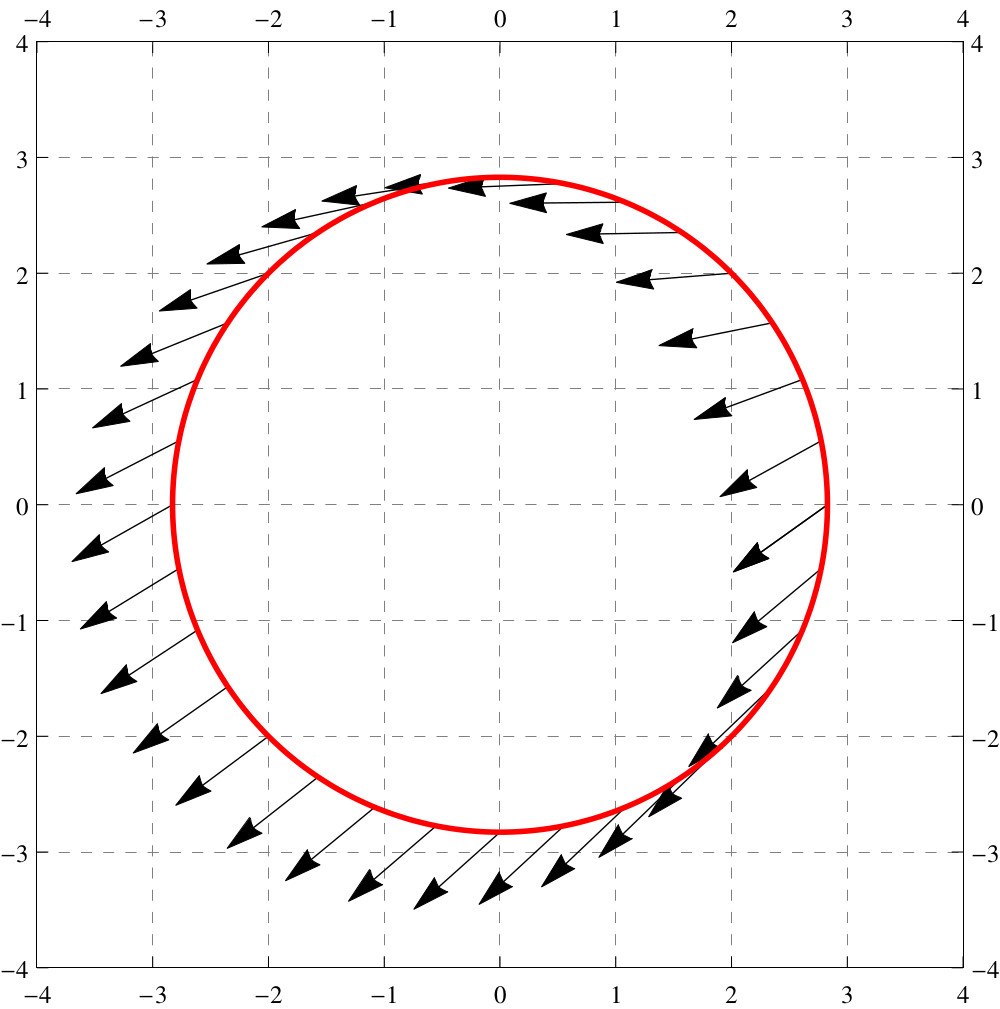
It is the last two facts that we will think about now. Below we see level curves for some function $F:\R ^2\to \R$ along with a constraining curve that we will call $S$ :

Let’s add vectors to our graph that point in the direction of $\grad F(x,y)$ . Since we know that the gradient vector is perpendicular to level curves, we can do this without computation.

If for some point $(x,y)$ on $S$ the gradient $\grad F(x,y)$ points in the “general” direction of the tangent vectors of $S$ , then $(x,y)$ cannot give an extremal value of $F$ , as moving along $S$ will either increase or decrease the value of $F$ . Here’s the upshot:

The only candidates for local extrema occur when the gradient of $F$ is perpendicular to $S$ .

How do we find these points? To do this, we will imagine that $S$ is a level curve for some other function $G:\R ^2\to \R$ , and define $S$ as: $S = \{(x,y):G(x,y)= c\}$ now, the candidates for extrema of $F$ when constrained to a curve $S$ are found by finding $(x,y)$ such that $\grad F(x,y) = \lambda \cdot \grad G(x,y)$ since $(x,y)$ that satisfy this equation are those where the gradient vectors of $F$ are perpendicular to the level curve $G(x,y)= c$ . This is the essence of the method of Lagrange multipliers.

Lagrange Multipliers Let $F:\R ^n\to \R$ , $G:\R ^n\to \R$ , $\grad G(\vec {x}) \ne \vec {0}$ , and let $S$ be the constraint, or level set, $S = \{\vec {x}: G(\vec {x}) = c\}$ If $F$ has extrema when constrained to $S$ at $\vec {x}$ , then $\grad F(\vec {x}) = \lambda \cdot \grad G(\vec {x})$ for some number $\lambda$ .

The first step for solving a constrained optimization problem using the method of Lagrange multipliers is to write down the equations needed to solve the problem.

Let $F(x,y) = xy$ and let $L$ the set $L = \{(x,y):(x^2+y^2)^2 = x^2-y^2\}$ Write down the three equations one must solve to find the extrema of $F$ when constrained to $L$ .

First set $G(x,y)= (x^2+y^2)^2 - x^2 +y^2$ . Now $L$ is the level curve $G(x,y) =\answer [given]{0}$ . We must write down: $\begin{align*} \grad F(x,y) &= \lambda \cdot \grad G(x,y)\\ (x^2+y^2)^2 &= x^2-y^2 \end{align*}$ Unpacking these formulas we find: $\begin{align*} y &= \lambda \cdot \left(\answer[given]{4x(x^2+y^2)-2x}\right)\\ x &= \lambda \cdot \left(\answer[given]{4y(x^2+y^2)+2y}\right)\\ (x^2+y^2)^2 &= \answer[given]{x^2-y^2} \end{align*}$ Solving these equations for $x$ and $y$ will give us our candidates for the extrema of $F$ on the set $L$ .

The constraint curve used in the example above is called the lemniscate of Bernoulli.

Working with geometry

Lagrange multipliers tell us that to maximize a function $F:\R ^2\to \R$ along a curve defined by $G(x,y) = c$ , we need to find where $\grad F$ is perpendicular to $G$ . In essence we are detecting geometric behavior using the tools of calculus.

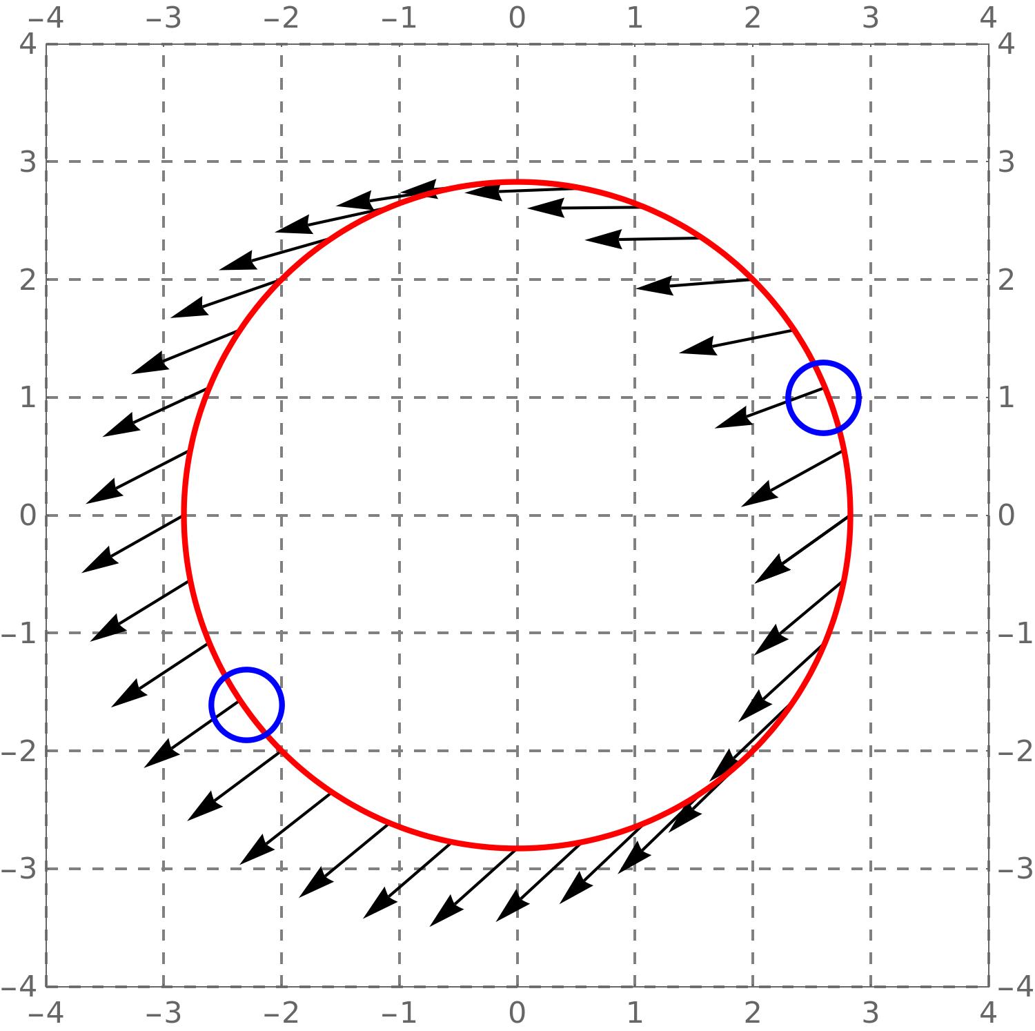
Below we have plotted a curve $G(x,y) = c$ along with $\grad F$ .

Find the candidates for the maximum and minimum values for $F$ when restricted to $G(x,y) = c$ .

At the candidates for the extrema, we know that the gradient vector of $F$ must be parallelperpendicular to the curve $G(x,y) = c$ . Hence we see that the points $(x,y)\approx \left (\answer [given,tolerance=.3]{2.6},\answer [given,tolerance=.3]{1}\right )$ and $(x,y)\approx \left (-2.3,\answer [given,tolerance=.3]{-1.6}\right )$ are our candidates for extrema.

At these points,

the gradient vector for $G$ are parallel to the gradient vectors for $F$ .

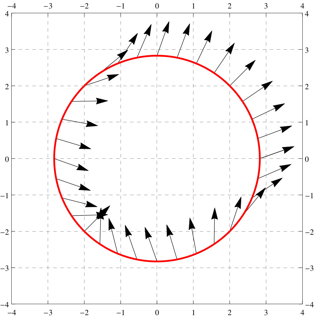
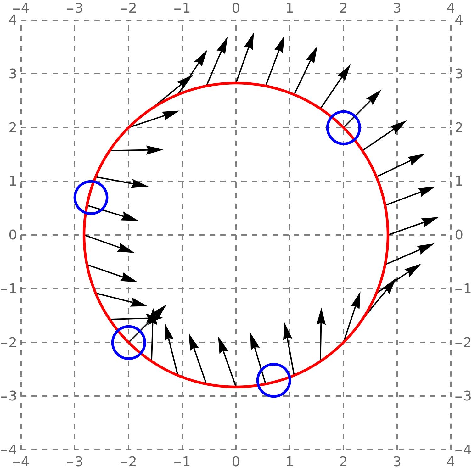
Below we have plotted a curve $G(x,y) = c$ along with $\grad F$ .

Find the candidates for the maximum and minimum values for $F$ when restricted to $G(x,y) = c$ .

At the candidates for the extrema, we know that the gradient vector of $F$ must be parallelperpendicular to the curve $G(x,y) = c$ . Hence we see that the points $\begin{align*} (x,y) &= \left(\answer[given]{2},2\right)\\ (x,y) &= \left(-2,\answer[given]{-2}\right)\\ (x,y) &\approx \left(\answer[given,tolerance=.3]{0.7},-2.7\right)\\ (x,y) &\approx \left(-2.7,\answer[given,tolerance=.3]{0.7}\right) \end{align*}$ are our candidates for extrema.

At these points,

the gradient vector for $G$ are parallel to the gradient vectors for $F$ .

Working with algebra

We’ll start with an example we did in our last section.

Let $F(x,y) = 4x^3+4y^2-4x$ and let $C$ the set $C = \{(x,y):x^2 + y^2 =1\}$ Find the maximum and minimum values of $F$ on $C$ .

Start by setting $G(x,y) = x^2 + y^2$ . The set $C$ is now the level curve $G(x,y) = \answer [given]{1}$ . Now compute: $\grad F(x,y) = \lambda \cdot \grad G(x,y)$ Write with me: $\vector {\answer [given]{12x^2-4},\answer [given]{8y}} = \lambda \cdot \vector {\answer [given]{2x},\answer [given]{2y}}$ Breaking this vector equation into components, and adding in the constraint equation, the method of Lagrange multipliers gives us three equations and three unknowns: $\begin{align*} \answer[given]{12x^2-4} &= \lambda 2x\\ \answer[given]{8y} &= \lambda 2y\\ \answer[given]{x^2 + y^2} &= 1 \end{align*}$ To solve this system of equations, first note that if $y = 0$ , then $x=\pm \answer [given]{1}$ . This gives us two candidates for extrema: $\left (1,\answer [given]{0}\right ) \quad \text {and}\quad \left (-1,\answer [given]{0}\right )$ Now proceed assuming that $y\ne 0$ . Looking at the second equation $8y = \lambda 2y$ we can divide both sides by $2y$ to see that $\lambda = \answer [given]{4}$ . Now we see that: $\begin{align*} 12x^2-4 &= \answer[given]{8x}\\ 3x^2-2x-1 &=0 \end{align*}$ Solving this quadratic equation for $x$ we find $x = \answer [given]{-1/3} \quad \text {and}\quad x = 1$ Now use the constraint equation $x^2 + y^2 =1$ to find $y$ -values. From this we gain two more candidate for an extrema: $\left (\frac {-1}{3},\answer [given]{\frac {-\sqrt {8}}{3}}\right ) \quad \text {and}\quad \left (\answer [given]{\frac {-1}{3}},\frac {\sqrt {8}}{3}\right )$ Plugging these points back into $F$ , we find that the minimum value of $F$ on $C$ is $\answer [given]{0}$ and the maximum value is $\answer [given]{128/27}$ .

Lagrange multipliers help out when when constraint set is given by an implicit function. Let’s see this in an example.

Let $F(x,y) = x^2+2y^2-28x+51$ and let $M$ the set $M = \{(x,y):y^2=x^3+1\}$ Find the maximum and minimum values of $F$ on $M$ .

Start by setting $G(x,y) = x^3+1-y^2$ . The set $M$ is now the level curve $G(x,y) = 0$ . Now compute: $\grad F(x,y) = \lambda \cdot \grad G(x,y)$ Write with me: $\vector {\answer [given]{2x-28},\answer [given]{4y}} = \lambda \cdot \vector {\answer [given]{3x^2},\answer [given]{-2y}}$ Breaking this vector equation into components, and adding in the constraint equation, the method of Lagrange multipliers gives us three unknowns: $\begin{align*} 2x-28 &= \lambda 3x^2\\ 4y &= -\lambda 2y\\ \answer[given]{x^3 + 1} &= y^2 \end{align*}$ To solve this system of equations, first note that if $y = 0$ , then $x=\answer [given]{-1}$ . This gives us our first candidate for an extrema: $\left (\answer [given]{-1},\answer [given]{0}\right )$ Now proceed assuming that $y\ne 0$ . Looking at the second equation $4y = -\lambda 2y$ we can divide both sides by $-2y$ to see that $\lambda = \answer [given]{-2}$ . Now we see that: $\begin{align*} 2x-28&= -6x^2\\ 3x^2+x-14 &=0 \end{align*}$ Solving this quadratic equation for $x$ we find $x = \answer [given]{-7/3} \quad \text {and}\quad x = 2$ Now use the constraint equation $x^3+1=y^2$ to find $y$ -values. If $x$ is $\answer [given]{-7/3}$ , then $y$ is not a real number, so we will discard this solution. If $x=\answer [given]{2}$ , then $y=\pm \answer [given]{3}$ . From this we gain two more candidate for an extrema: $\left (\answer [given]{2},\answer [given]{-3}\right ) \quad \text {and}\quad \left (2,3\right )$ Plugging these points back into $F$ , we find that the minimum value of $F$ on $M$ is $\answer [given]{17}$ and the maximum value is $\answer [given]{80}$ .

The constraint curve used in the example above is called a Mordell curve. The Mordell curve is a type of elliptic curve, a central object of study in number theory and cryptography. For much more information on the Mordell curve, see this paper by Keith Conrad.

The method of Lagrange multipliers gives a unified method for solving a large class of constrained optimization problems, and hence is used in many areas of applied mathematics.

For some interesting extra reading check out: