Curl and Green’s Theorem

$\newenvironment {prompt}{}{} \newcommand {\ungraded }[0]{} \newcommand {\todo }[0]{} \newcommand {\oiint }[0]{{\large \bigcirc }\kern -1.56em\iint } \newcommand {\mooculus }[0]{\textsf {\textbf {MOOC}\textnormal {\textsf {ULUS}}}} \newcommand {\npnoround }[0]{\nprounddigits {-1}} \newcommand {\npnoroundexp }[0]{\nproundexpdigits {-1}} \newcommand {\npunitcommand }[1]{\ensuremath {\mathrm {#1}}} \newcommand {\RR }[0]{\mathbb R} \newcommand {\R }[0]{\mathbb R} \newcommand {\N }[0]{\mathbb N} \newcommand {\Z }[0]{\mathbb Z} \newcommand {\sagemath }[0]{\textsf {SageMath}} \newcommand {\d }[0]{\,d} \newcommand {\l }[0]{\ell } \newcommand {\ddx }[0]{\frac {d}{\d x}} \newcommand {\zeroOverZero }[0]{\ensuremath {\boldsymbol {\tfrac {0}{0}}}} \newcommand {\inftyOverInfty }[0]{\ensuremath {\boldsymbol {\tfrac {\infty }{\infty }}}} \newcommand {\zeroOverInfty }[0]{\ensuremath {\boldsymbol {\tfrac {0}{\infty }}}} \newcommand {\zeroTimesInfty }[0]{\ensuremath {\small \boldsymbol {0\cdot \infty }}} \newcommand {\inftyMinusInfty }[0]{\ensuremath {\small \boldsymbol {\infty -\infty }}} \newcommand {\oneToInfty }[0]{\ensuremath {\boldsymbol {1^\infty }}} \newcommand {\zeroToZero }[0]{\ensuremath {\boldsymbol {0^0}}} \newcommand {\inftyToZero }[0]{\ensuremath {\boldsymbol {\infty ^0}}} \newcommand {\numOverZero }[0]{\ensuremath {\boldsymbol {\tfrac {\#}{0}}}} \newcommand {\dfn }[0]{\textbf } \newcommand {\unit }[0]{\mathop {}\!\mathrm } \newcommand {\eval }[1]{\bigg [ #1 \bigg ]} \newcommand {\seq }[1]{\left ( #1 \right )} \newcommand {\epsilon }[0]{\varepsilon } \newcommand {\phi }[0]{\varphi } \newcommand {\iff }[0]{\Leftrightarrow } \DeclareMathOperator {\arccot }{arccot} \DeclareMathOperator {\arcsec }{arcsec} \DeclareMathOperator {\arccsc }{arccsc} \DeclareMathOperator {\si }{Si} \DeclareMathOperator {\scal }{scal} \DeclareMathOperator {\sign }{sign} \newcommand {\arrowvec }[1]{{\overset {\rightharpoonup }{#1}}} \newcommand {\vec }[1]{{\overset {\boldsymbol {\rightharpoonup }}{\mathbf {#1}}}\hspace {0in}} \newcommand {\point }[1]{\left (#1\right )} \newcommand {\pt }[1]{\mathbf {#1}} \newcommand {\Lim }[2]{\lim _{\point {#1} \to \point {#2}}} \DeclareMathOperator {\proj }{\mathbf {proj}} \newcommand {\veci }[0]{{\boldsymbol {\hat {\imath }}}} \newcommand {\vecj }[0]{{\boldsymbol {\hat {\jmath }}}} \newcommand {\veck }[0]{{\boldsymbol {\hat {k}}}} \newcommand {\vecl }[0]{\vec {\boldsymbol {\l }}} \newcommand {\uvec }[1]{\mathbf {\hat {#1}}} \newcommand {\utan }[0]{\mathbf {\hat {t}}} \newcommand {\unormal }[0]{\mathbf {\hat {n}}} \newcommand {\ubinormal }[0]{\mathbf {\hat {b}}} \newcommand {\dotp }[0]{\bullet } \newcommand {\cross }[0]{\boldsymbol \times } \newcommand {\grad }[0]{\boldsymbol \nabla } \newcommand {\divergence }[0]{\grad \dotp } \newcommand {\curl }[0]{\grad \cross } \newcommand {\lto }[0]{\mathop {\longrightarrow \,}\limits } \newcommand {\bar }[0]{\overline } \newcommand {\surfaceColor }[0]{violet} \newcommand {\surfaceColorTwo }[0]{redyellow} \newcommand {\sliceColor }[0]{greenyellow} \newcommand {\vector }[1]{\left \langle #1\right \rangle } \newcommand {\sectionOutcomes }[0]{} \newcommand {\HyperFirstAtBeginDocument }[0]{\AtBeginDocument } \newcommand {\arraystretch }[0]{1.2}$

Green’s Theorem is a fundamental theorem of calculus.

A fundamental object in calculus is the derivative. However, there are different derivatives for different types of functions, an in each case the interpretation of the derivative is different. Check out the table below:


Function	Example	Derivative	Interpretation


explicit curve	$y = x^2$	$\dd [y]{x} = 2x$	slope of the tangent line

vector-valued function	$\vec {p}(t) = \vector {t,t^2}$	$\vec {p}'(t) = \vector {1,2t}$	tangent vector

explicit surface	$z = F(x,y) = x^2 -y$	$\grad F(x,y)$	the vector that points in the initial direction of greatest increase of $z$

implicit curve (level curve)	$0 = \underbrace {x^2 - y}_{G(x,y)}$	$\grad G(x,y)$	gradient vectors are orthogonal to level sets

In this section we will learn the fundamental derivative for two-dimensional vector fields, as well as a new fundamental theorem of calculus.

The curl of a vector field

Calculus has taught us that knowing the derivative of a function $f:\R \to \R$ can tell us important information about the function. In a similar way we have seen that if we wish to understand a function of several variables $F:\R ^n\to \R$ , then the gradient, $\grad F$ , contains similar useful information. If you have a vector field $\vec {F}:\R ^n\to \R ^n,$ we now ask: “what is the natural analogue of a derivative in this setting?” When the vector field is two or three-dimensional, the curl is the analogue of the derivative that we are looking for:

In two dimensions, given a vector field $\vec {F}:\R ^2\to \R ^2$ , where $\vec {F}(x,y) = \vector {M(x,y),N(x,y)}$ the (scalar) curl is given by $\curl \vec F = \pp [N]{x}-\pp [M]{y}.$ In three dimensions, given a vector field $\vec {F}:\R ^3\to \R ^3$ , where $\vec {F}(x,y,z) = \vector {U(x,y,z),V(x,y,z),W(x,y,z)}$ the curl is given by $\begin{align*} \curl \vec F &= \det \begin{bmatrix} \veci & \vecj & \veck \\ \pp{x} & \pp{y} & \pp{z}\\ U & V & W \end{bmatrix}\\ &= \veci\left(\pp[W]{y}-\pp[V]{z}\right)- \vecj\left(\pp[W]{x}-\pp[U]{z}\right)+ \veck\left(\pp[V]{x}-\pp[U]{y}\right). \end{align*}$ Other authors sometimes use the notation $\mathop {\mathrm {rot}}\vec {F}$ for the scalar curl of a two-dimensional vector field $\vec {F}:\R ^2\to \R ^2$ , and $\mathop {\mathrm {curl}}\vec {F}$ for the curl of a three-dimensional vector field $\vec {F}:\R ^3\to \R ^3$ .

In two dimensions, is $\curl \vec {F}$ a number or a vector?

number. vector.

In three dimensions, is $\curl \vec {F}$ a number or a vector?

number. vector.

Consider the vector field $\vec {F}(x,y) = \vector {-y,x}$ . Compute: $\curl \vec {F}(x,y) \begin {prompt}= \answer {2}\end {prompt}$

Consider the vector field $\vec {F}(x,y,z) = \vector {-z,x,y}$ . Compute: $\curl \vec {F}(x,y,z) \begin {prompt} = \vector {\answer {1},\answer {-1},\answer {1}} \end {prompt}$

Now for something you’ve seen before, but in a different form.

Let $F:\R ^2\to \R$ . Compute: $\curl \grad F(x,y) \begin {prompt}= \answer {0}\end {prompt}$

Let $F:\R ^3\to \R$ . Compute: $\curl \grad F(x,y,z) \begin {prompt}= \vector {\answer {0},\answer {0},\answer {0}}\end {prompt}$

When $\curl \vec {F} = \vec {0}$ , then you know:

$\vec {F}$ is a gradient field. $\vec {F}$ is a conservative field. $\vec {F}:\R ^3\to \R ^3$ .

You can be assured that $\vec {F}:\R ^3\to \R ^3$ , since $\vec {0}$ is a vector. We only know a definition for curl in two and three dimensions; however, the two-dimensional definition is a scalar, not a vector. So if $\curl \vec {F} = \vec {0}$ , then $\vec {F}:\R ^3\to \R ^3$ .

What does the curl measure?

The curl of a vector field measures the rate that the direction of field vectors “twist” as $x$ and $y$ change. Imagine the vectors in a vector field as representing the current of a river. A positive curl at a point tells you that a “beach-ball” floating at the point would be rotating in a counterclockwise direction. A negative curl at a point tells you that a “beach-ball” floating at the point would be rotating in a clockwise direction. Zero curl means that the “beach-ball” would not be rotating. Below we see our “beach-ball” with two field vectors. If $\vec {F}(x,y) = \vector {M(x,y),N(x,y)}$

we see that the right field vector is larger than the left, thus giving the “beach-ball” a counterclockwise rotation. In an entirely similar way, if we have

we see that the bottom field vector is larger than the top, thus giving the “beach-ball” a counterclockwise rotation. Thus the curl combines $\pp [N]{x}$ and $-\pp [M]{y}$ $\curl \vec {F} = \pp [N]{x} - \pp [M]{y}$ to obtain the local rotation of the field. The most obvious example of a vector field with nonzero curl is $\vec {F}(x,y) = \vector {-y,x}$ .

In essence, the scalar curl measures how the magnitude of the field vectors change as you move to the right, in a direction perpendicular to the direction of the field vectors:

And:

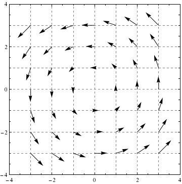
In our next example, we see a field that has local rotation (nonzero curl) but does not have global rotation.

Consider the following vector field $\vec {F}$ :

Setting $\d x = 1$ and $\d y = 1$ , estimate: $\curl \vec {F}(\vec {a})$

First note that one should imagine a vector at every point. We’ll assume that the magnitudes of the vectors are constant along vertical lines. Set $\vec {F}(x,y) = \vector {M(x,y),N(x,y)}$ . To estimate $\pp [N]{x}$ , we examine the change in $N(x,1)$ between $x=1$ and $x=2$ : $\frac {N(2,1) - N(1,1)}{2-1} = \answer [given]{1}$ and we should also check the change of $N(x,1)$ between $x=2$ and $x=3$ : $\frac {N(3,1) - N(2,1)}{3-2} = \answer [given]{1}$ Averaging these values together we find $\pp [N]{x} \approx \answer [given]{1}$ To estimate $\pp [M]{y}$ , we examine the change in $M(2,y)$ between $y=0$ and $y=1$ : $\frac {M(2,1) - M(2,0)}{1-0} = \answer [given]{0}$ and we should also check the change of $M(2,y)$ between $y=1$ and $y=2$ : $\frac {M(2,2) - M(2,1)}{2-1} = \answer [given]{0}$ Averaging these values together we find $\pp [M]{y} \approx \answer [given]{0}$ So we approximate $\curl \vec {F}(\vec {a})\approx \answer [given]{1}.$ So field above example does not have global rotation, but it does have local rotation.

Now we’ll show you a field that has global rotation but no local rotation!

Consider the vector field $\vec {F}(x,y) = \vector {\frac {-y}{x^2+y^2},\frac {x}{x^2+y^2}}$

Compute: $\curl \vec {F}(x,y)$

In this case, $\curl \vec {F}(x,y) =\answer [given]{0}$ when $\vector {x,y}\ne \vec {0}$ . At $\vec {0}$ , the curl of the vector field is zeroinfinityundefined , and hence this field is not a gradient field. This field has global rotation, but it does not have local rotation.

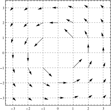
Finally, we’ll show you a field that has global rotation with local rotation in the opposite direction!

Consider the vector field $\vec {F}(x,y) = \vector {\frac {-y}{(x^2+y^2)^{3/2}},\frac {x}{(x^2+y^2)^{3/2}}}$

Compute: $\curl \vec {F}(x,y)$

In this case, $\curl \vec {F}(x,y) =\answer [given]{\frac {-1}{(x^2+y^2)^{3/2}}}$ when $\vector {x,y}\ne \vec {0}$ . Note, this is positivenegative for all values of $x$ and $y$ . This corresponds to local rotation in the clockwisecounterclockwise direction. This field has global rotation in the clockwisecounterclockwise direction, but has local rotation in the clockwisecounterclockwise direction.

Curl in three dimensions

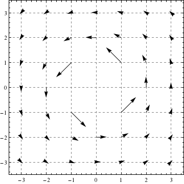
In this section we introduce curl in three dimensions. You already know how to compute it:

$\begin{align*} \curl \vec F &= \det \begin{bmatrix} \veci & \vecj & \veck \\ \pp{x} & \pp{y} & \pp{z}\\ U & V & W \end{bmatrix}\\ &= \veci\left(\pp[W]{y}-\pp[V]{z}\right)- \vecj\left(\pp[W]{x}-\pp[U]{z}\right)+ \veck\left(\pp[V]{x}-\pp[U]{y}\right). \end{align*}$ What does it mean? Well first of all, in three dimensions, curl is a vector. It points along the axis of rotation for a vector field. You should think of a tornado:

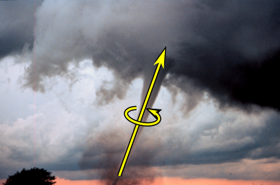
Here the vector pointing up is supposed to be the curl of the tornado.

At this point we only know how to take the derivative (via the curl) of a vector field of two or three dimensions. You can take another course to learn more about derivatives of $n$ -dimensional vector fields.

A new fundamental theorem of calculus

Recall that a fundamental theorem of calculus says something like:

To compute a certain sort of integral over a region, we may do a computation on the boundary of the region that involves one fewer integrations.

In the single variable case we have:

With line integrals we have:

We now introduce a new fundamental theorem of calculus involving the curl. It’s called Green’s Theorem:

Green’s Theorem If the components of $\vec {F}:\R ^2\to \R ^2$ have continuous partial derivatives on a closed region $R$ where $C$ is a boundary of $R$ and $\vec {p}(t)$ parameterizes $C$ in a counterclockwise direction with the interior on the left,

then $\iint _R \curl \vec {F}\d A = \oint _C \vec {F}\dotp \d \vec {p}$

Let $C$ be the rectangle with corners $(2,-1)$ , $(2,4)$ , $(3,4)$ , and $(3,-1)$ . Compute: $\oint _C \frac {\sin (x)}{x} \d x + x^2 \d y$

We’ll use Green’s Theorem to squash this scary integral with ease. First note that if we imagine $\oint _C \frac {\sin (x)}{x} \d x + x^2 \d y = \oint _C\vec {F}\dotp \d \vec {p}$ we set: $\vec {F}(x,y) = \vector {\answer [given]{\frac {\sin (x)}{x}},\answer [given]{x^2}}$ Further note that our field is continuous on the interior of the rectangle. Thus we may apply Green’s Theorem! Write with me now, $\curl \vec {F}(x,y) = \answer [given]{2x}$ So by Green’s Theorem $\oint _C \frac {\sin (x)}{x} \d x + x^2 \d y = \int _{\answer [given]{-1}}^{\answer [given]{4}}\int _{\answer [given]{2}}^{\answer [given]{3}} \answer [given]{2x}\d x\d y$ Now, keep writing with me, $\begin{align*} \int_{\answer[given]{-1}}^{\answer[given]{4}}\int_{\answer[given]{2}}^{\answer[given]{3}} \answer[given]{2x}\d x\d y &= \int_{\answer[given]{-1}}^{\answer[given]{4}} \answer[given]{5} \d y\\ &= \answer[given]{25}. \end{align*}$ The upshot is that we were able to use Green’s Theorem to transform a tedious integral into a trivial one.

Suppose that the curl of a vector field $\vec {F}:\R ^2\to \R ^2$ is constant, $\curl \vec {F} = 3$ .

If $\int _{C_1} \vec {F} \dotp \d \vec {p} = 20$ estimate $\int _{C_2} \vec {F}\dotp \d \vec {p} \begin {prompt} = \answer {46} \end {prompt}$

Use Green’s Theorem.

How is Green’s Theorem a fundamental theorem of calculus? Well consider this:

The “hand-wavey” reason this works is given by the picture below:

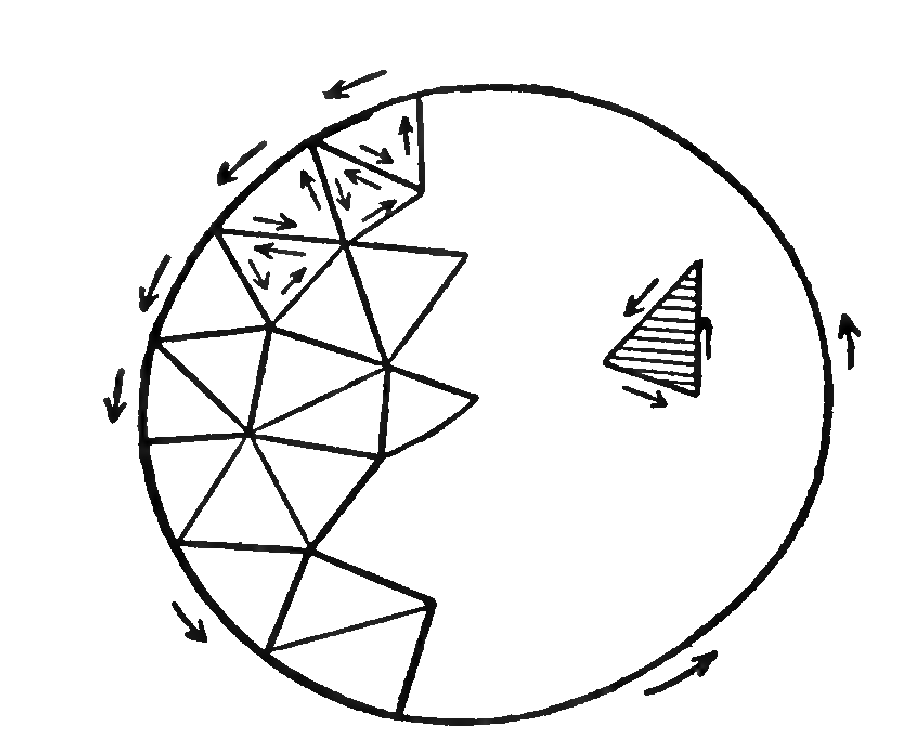
Basically, $\curl \vec {F}\d A$ measures the circulation (local rotation) in every little triangle above. Lining each of these little triangles up, we see that the accumulation of this circulation is measured by the flow of the vector field along the boundary, and this is measured by: $\oint _C \vec {F}\dotp \d \vec {p}$ Green’s Theorem is our shiny new fundamental theorem of calculus. We’ll be talking about it in the next two sections too!

Strategy for evaluating line integrals

At this point we have three ways to evaluating two-dimensional line integrals:

Direct computation.
The Fundamental Theorem of Line Integrals.
Green’s Theorem.

How do you know which method to use? Here are some rules of thumb.

Identify the field With line integrals, we must have a vector field. You must identify this vector field.

Compute the scalar curl of the field If the scalar curl is zero, then the field is a gradient field. If the scalar curl is “simple” then proceed on, and you might want to use Green’s Theorem.

Is the boundary a closed curve? If the field is a gradient field and the curve is closed, then the integral is zero (by both the Fundamental Theorem of Line Integrals and Green’s Theorem).

If the boundary is not a closed curve and the curl is not zero, you must use direct computation.

If the curl is simple and the boundary is a closed curve, then maybe use Green’s Theorem.

The shape of things to come

Recalling that $C^\infty (A,B)$ is the set of differentiable functions from $A$ to $B$ where all of the derivatives are continuous, we can make the following “chain” of derivatives:

$\underbrace {C^{\infty }(\R ^2,\R )}_{\text {surfaces}} \overset {\grad }{\to }\underbrace {C^\infty (\R ^2,\R ^2)}_{\text {vector fields}} \overset {\curl }{\to }\underbrace {C^\infty (\R ^2,\R )}_{\text {surfaces}}$ Moreover, by the Clairaut gradient test, the scalar curl of the gradient vector is zero. Given a function $F:\R ^2\to \R$ , we can follow $F$ through the chain to see what happens:

This is nothing more than a fancy way to say that $\curl \grad F = 0$ . However, we also have our two new fundamental theorems of calculus: The Fundamental Theorem of Line Integrals (FTLI), and Green’s Theorem. These theorems also fit on this sort of diagram:

The Fundamental Theorem of Line Integrals is in some sense about “undoing” the gradient. Green’s Theorem is in some sense about “undoing” the scalar curl. Are there more fundamental theorems of calculus? Absolutely, read on young mathematician!