You are about to erase your work on this activity. Are you sure you want to do this?
Updated Version Available
There is an updated version of this activity. If you update to the most recent version of this activity, then your current progress on this activity will be erased. Regardless, your record of completion will remain. How would you like to proceed?
Mathematical Expression Editor
Divergence measures the rate field vectors are expanding at a point.
While the gradient and curl are the fundamental “derivatives” in two dimensions,
there is another useful measurement we can make. It is called divergence. It measures
the rate field vectors are “expanding” at a given point.
1 The divergence of a vector field
Let’s state the definition:
Given a vector field \(\vec {F}:\R ^n\to \R ^n\), where
As we’ve already said, divergence measures the rate field vectors are expanding at a
point. To be more explicit, the divergence measures how the magnitude of
the field vectors change as you move in the direction of the field vectors:
And:
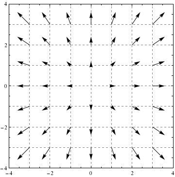
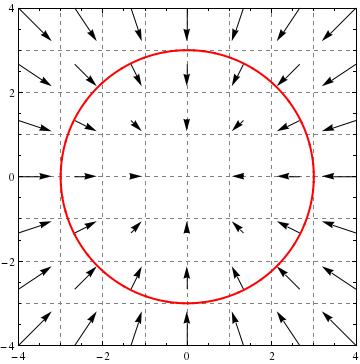
The most obvious example of a vector field with nonzero divergence is \(\vec {F}(x,y)= \vector {x,y}\):
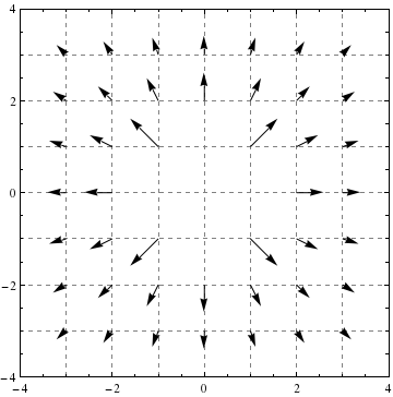
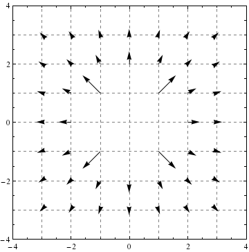
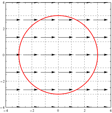
On the other hand, recall that a radial vector field is a field of the form \(\vec {F}:\R ^n\to \R ^n\)
where
Let \(\vec {F}:\R ^2\to \R ^2\) be a vector field, \(\vec {p}:\R \to \R ^2\) be a smooth vector valued function tracing a curve \(C\) exactly
once as \(t\) runs from \(a\) to \(b\),
measures the accumulated flow of a vector field along a
curve. We see this because \(\vec {F}\dotp \vec {p}'\) measures how “aligned” field vectors are with the
direction of the path \(\vec {p}\). On the other hand, if we set
\[ \vec {n}(t) = \vector {y(t),-x(t)} \]
then for any given value of \(t\), \(\vec {n}'(t)\) is
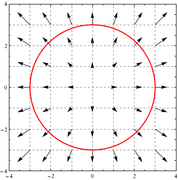
a vector that is orthogonal to \(\vec {p}'(t)\). Moreover, given a closed curve, where \(\vec {p}(t)\) is
parameterized with the interior on the left, \(\vec {n}'(t)\) points outward. Below we see a
curve \(\vec {p}(t)\) along with some tangent vectors \(\vec {p}'(t)\) and some outward normal vectors \(\vec {n}'(t)\):
Since \(\vec {F}\dotp \vec {n}'\) measures
how “aligned” field vectors are with vectors orthogonal to the direction of the path,
the integral
measures the flow of a vector field across a curve. Some folks call this a flux
integral. Since \(\d x = x'(t)\d t\) and \(\d y = y'(t)\d t\), we may write \(\oint _C \vec {F}\dotp \d \vec {n}\) as
this leads us to the flux form of Green’s Theorem:
Green’s Theorem If the components of \(\vec {F}:\R ^2\to \R ^2\) have continuous partial derivatives and \(C\) is a
boundary of a closed region \(R\) and \(\vec {p}(t) = \vector {x(t),y(t)}\) parameterizes \(C\) in a counterclockwise direction with
the interior on the left, and \(\vec {n}(t) = \vector {y(t),-x(t)}\), then
![[Picture]](digInDivergenceAndGreensTheorem.online-a934edc4203b81bed98c134e4d2be2ab.svg)
![[Picture]](digInDivergenceAndGreensTheorem.online-a7f76f1ef6c35a33867d3b2875c74cee.svg)
![[Picture]](digInDivergenceAndGreensTheorem.online-e543d29a31cabcdc353dc754b377ef62.svg)
![[Picture]](digInDivergenceAndGreensTheorem.online-68d8e55188d6a2b83313aea9fe4c712b.svg)
![[Picture]](digInDivergenceAndGreensTheorem.online-2e8c4b07a814fc116b451065bbdd3aee.svg)