You are about to erase your work on this activity. Are you sure you want to do this?
Updated Version Available
There is an updated version of this activity. If you update to the most recent version of this activity, then your current progress on this activity will be erased. Regardless, your record of completion will remain. How would you like to proceed?
Mathematical Expression Editor
We introduce partial derivatives and the gradient vector.
Given a function \(F:\R ^n \to \R \), it is often useful to differentiate with respect to a single variable
and hold the other variables as constants. One way to think of a function of several
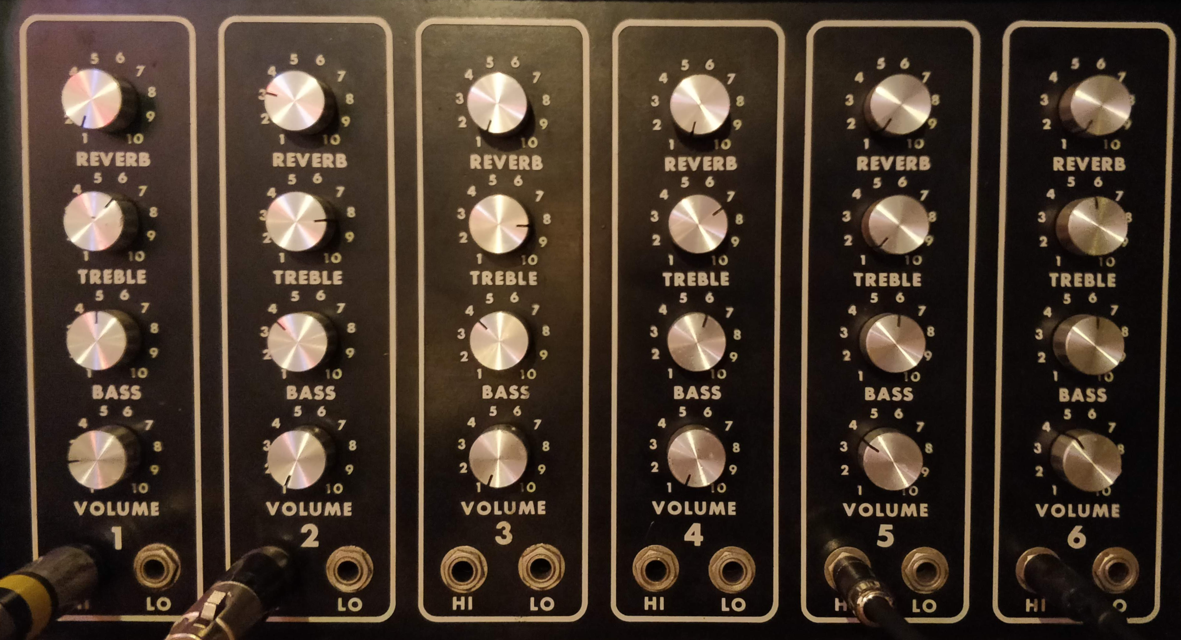
variables is as a “machine” with lots of knobs:
One way to try and understand
the machine above would be to hold all but one of the knobs constant, and see what
happens when you “wiggle” a single knob. As a explicit example, let
\[ F(x,y) = x^2+2y^2 \]
Here \(F\) is
our “machine” and the variables \(x\) and \(y\) are the “knobs.” Fixing \(y=2\), allows us
to focus our attention to all points on the surface where the \(y\)-value is \(2\),
We can now focus our
attention on the curve
and differentiate this curve purely with respect to \(x\). In a similar way, we could fix \(x\)
and differentiate with respect to \(y\).
Given a function \(F:\R ^n\to \R \), the partial derivative of \(F\) with respect to the \(i\)th variable is
denoted:
We have shown how to compute a partial derivative, but it may still not be clear
what a partial derivative means. Given \(z=F(x,y)\), \(F^{(1,0)}(x,y)\) measures the rate at which \(z\) changes as only
\(x\) varies: \(y\) is held constant.
Imagine standing in a rolling meadow, then beginning to walk due east. Depending
on your location, you might walk up, sharply down, or perhaps not change elevation
at all. This is similar to measuring \(\pp [z]{x}\): you are moving only east (in the \(x\)-direction) and
not north/south at all. Going back to your original location, imagine now walking
due north (in the \(y\)-direction). Perhaps walking due north does not change your
elevation at all. This is analogous to \(\pp [z]{y}=0\): \(z\) does not change with respect to \(y\). We can
see that \(\pp [z]{x}\) and \(\pp [z]{y}\) do not have to be the same, or even similar, as it is easy to
imagine circumstances where walking east means you walk downhill, though
walking north makes you walk uphill. The next example helps us visualize
this.
Let \(F(x,y)=-x^2-\frac {y^2}{2}+xy+10\). Find \(F^{(1,0)}(2,1)\) and \(F^{(0,1)}(2,1)\).
Write with me
\[ \pp {x}F(x,y) = \answer [given]{-2x+y} \]
and
\[ \pp {y}F(x,y) = \answer [given]{-y+x} \]
Thus \(F^{(1,0)}(2,1) = \answer [given]{-3}\) and \(F^{(0,1)}(2,1) = \answer [given]{1}\).
Whenever we do a computation in mathematics, we should ask ourselves, “What does
this mean?”
Let \(F(x,y)=-x^2-\frac {y^2}{2}+xy+10\). What is the meaning of
First note that \(F(2,1) = \answer [given]{7.5}\). If \(F^{(1,0)}(2,1)=-3\), this means if one “stands” on the surface at the point \(\left (\answer [given]{2},\answer [given]{1},\answer [given]{7.5}\right )\) and
moves parallelorthogonal to the \(x\)-axis (so only the \(x\)-value changes, not the \(y\)-value),
then the instantaneous rate of change in \(z\) is \(\answer [given]{-3}\). Increasing the \(x\)-value will increasedecrease the \(z\)-value; decreasing the \(x\)-value will increasedecrease the
\(z\)-value.
If \(F^{(0,1)}(2,1)=1\), this means if one “stands” on the surface at the point \((\answer [given]{2},\answer [given]{1},\answer [given]{7.5})\) and moves parallelorthogonal to the \(y\)-axis (so only the \(y\)-value changes, not the \(x\)-value), then the
instantaneous rate of change in \(z\) is \(\answer [given]{1}\). Increasing the \(y\)-value will increasedecrease the \(z\)-value; decreasing the \(y\)-value will increasedecrease the \(z\)-value.
Finally, since the
magnitude of \(\pp [F]{x}\) is greater than the magnitude of \(\pp [F]{y}\) at \((2,1)\), the surface is “steeper” in the
\(x\)-direction than in the \(y\)-direction.
1 Estimating partial derivatives
Functions of several variables, especially ones that map \(\R ^2\to \R \) can be described
by a table of values or level curves. In either case we can estimate partial
derivatives by looking at
\[ \frac {\text {change in the output}}{\text {change in the variable}} \]
Let’s do an example to make this more clear.
Let \(F:\R ^2\to \R \)
be a differentiable function described by the following table of values:
Estimate \(F^{(1,0)}(2,6)\).
To estimate \(F^{(1,0)}(2,6)\), we
examine the change in \(F(x,6)\) between \(x=1\) and \(x=2\) and then between \(x=2\) and \(x=3\). We will then
average these estimates to find our answer. To start look between \(x=1\) and \(x=2\):
Let \(F:\R ^2\to \R \) be a differentiable function described by the following table of values:
Estimate \(F^{(0,1)}(2,6)\).
\[ F^{(0,1)}(2,6)\approx \answer {.5} \]
Work as we did
in the example above, finding two estimates and taking their averages.
We can also estimate partial derivatives by looking at level curves.
Let \(F:\R ^2\to \R \) be described by the level curves below:
The height of the level curve is marked on the curve, and we are given a point \((4,2)\).
Estimate \(F^{(1,0)}(4,2)\).
To estimate \(F^{(1,0)}(4,2)\), we examine the change between the level curve that \(\vec {p}\) is on
and the nearest level curve found by traveling on a line parallel to the \(x\)-axis.
Starting at \(\vec {p}\) and moving to the left on a line parallel to the \(x\)-axis, we see
Work as we did in the example above, finding two estimates and taking their
averages.
2 Combining partial derivatives
While a function \(f:\R \to \R \) only has one second derivative. However, functions \(F:\R ^2\to \R \) have \(4\)second
partial derivatives and functions \(F:\R ^3\to \R \) have \(9\)second partial derivatives! Don’t run off yet,
things get better.
Let \(F:\R ^n\to \R \) be continuous on an open set \(S\).
The second pure partial derivative of \(F\) with respect to \(x\) then \(x\) is
The notation \(F^{(1,1)}\) is ambiguous, it does not state which derivative should be
taken first. As we will see, in practice this is not too much of a problem.
Notice how above \(\frac {\partial ^2F}{\partial y\partial x}=\frac {\partial ^2F}{\partial x\partial y}\). The next theorem states that it is not a coincidence.
Mixed Partial Derivatives Let \(F:\R ^2\to \R \) be a function where
are continuous on an
open set \(S\). Then for each point \((x,y)\) in \(S\), \(\frac {\partial ^2F}{\partial y\partial x}=\frac {\partial ^2F}{\partial x\partial y}\). A similar result is true for functions \(F:\R ^n\to \R \).
Finding \(\frac {\partial ^2F}{\partial y\partial x}\) and \(\frac {\partial ^2F}{\partial x\partial y}\) independently and comparing the results provides a convenient way of
checking our work.
3 The gradient vector
Given a function \(F:\R ^n\to \R \), we often want to work with all of first partial derivatives
simultaneously. In this case, we will work with the vector:
As we will see, for
functions of several variables, this vector will play the role that the derivative did for
functions of a single variable. This vector is called the gradient vector.
Let \(F:\R ^n\to \R \) be a function whose first partial derivatives exist, the gradient
The upside-down triangle in the notation for the gradient sometimes called a del. It is
also known as a nabla. You can think of the \(\grad \) as the vector:
and hence when one
writes: \(\grad F\), you are literally distributing the \(F\) across the vector, just as a scalar acts on a
vector.
The gradient is defined at points in the domain where the partial derivatives are
defined. The gradient of a function of two variables lives in \(\R ^2\). The gradient of a
function of three variables lives in \(\R ^3\). Generally the gradient of a function of \(n\) variables
lives in \(\R ^n\). We can see this in the interactive below.
The gradient at each point is a vector pointing in the \((x,y)\)-plane.
Above, note that \(\grad F(x,y)\) is a vector whose components are
functions of \(x\) and \(y\), hence it is a vector-valued function. We can evaluate
functions at actual points in their domain. For instance, if \(\vec {p}= \vector {\pi /3,\pi /3}\) we compute:
![[Picture]](digInPartialDerivatives.online-ca005406abce86ddb6d1ff49d0f140d4.svg)
![[Picture]](digInPartialDerivatives.online-9eaa383f92b9e67b71ed226162ef2be2.svg)
![[Picture]](digInPartialDerivatives.online-bc0a48f7e3617410613fce947e17349d.svg)
![[Picture]](digInPartialDerivatives.online-31e76624a56e53fe7b7087852ea73976.svg)
![[Picture]](digInPartialDerivatives.online-d31735932ec4f58e3fcb143232551148.svg)
![[Picture]](digInPartialDerivatives.online-b9cadcdf1e064d605f4dced28cdf196b.svg)
![[Picture]](digInPartialDerivatives.online-a49f70507d7d2b7430e330e52357d7be.svg)
![[Picture]](digInPartialDerivatives.online-a5eb93842991e0ac3344969bdf06daae.svg)