In this section, we explore the graphs of secant, cosecant, and cotangent.
- What do the graphs of secant, cosecant, and cotangent look like?
- What are some important properties of these graphs? Where do they have asymptotes?
The Secant Function
We begin by investigating the secant function. Using the fact that , we note that anywhere , the value of is undefined. We record such instances in the following table by writing “”. At all other points, the value of the secant function is simply the reciprocal of the cosine function’s value. Since for all , it follows that for all (for which the secant’s value is defined).
Values of Secant in Quadrant I
Values of Secant in Quadrant II
Values of Secant in Quadrant III
Values of Secant in Quadrant IV
These tables help us identify trends in the secant function. The sign of matches the sign of and thus is positive in Quadrant I, negative in Quadrant II, negative in Quadrant III, and positive in Quadrant IV.
In addition, we observe that as -values in the first quadrant get closer to , gets closer to (while being always positive). Since the numerator of the secant function is always , having its denominator approach means that increases without bound as approaches from the left side. Once is slightly greater than in Quadrant II, the value of is negative (and close to zero). This makes the value of decrease without bound (negative and getting further away from ) for approaching from the right side, and results in having a vertical asymptote at . The periodicity and sign behavior of mean this asymptotic behavior of the secant function will repeat.
Plotting the data in the table along with the expected asymptotes and connecting the points intuitively, we see the graph of the secant function.
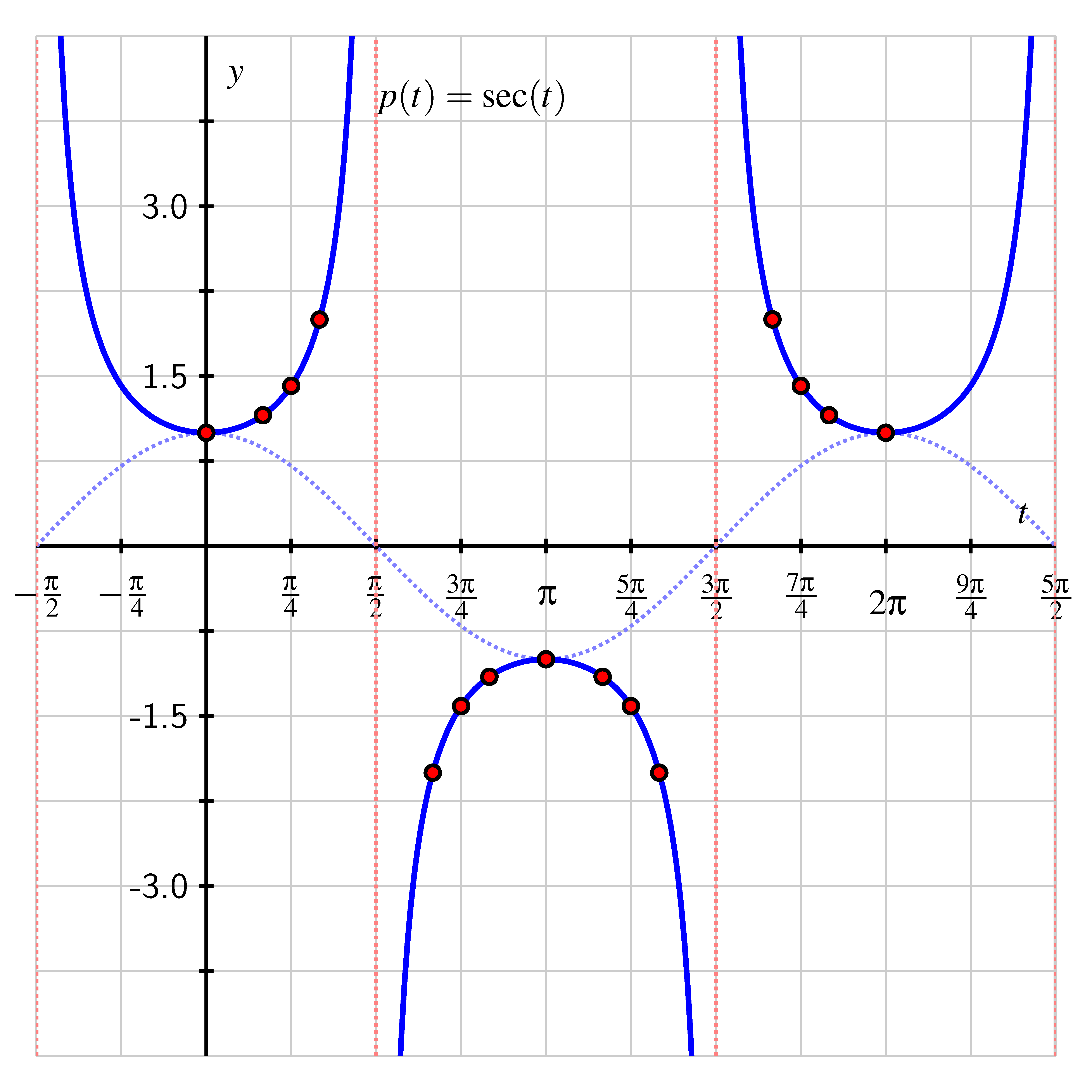
We see from both the table and the graph that the secant function has period . We summarize our recent work as follows.
For the function ,
- its domain is the set of all real numbers except where is any odd number;
- its range is the set of all real numbers such that ;
- its period is .
We can see the secant function in Desmos as well.
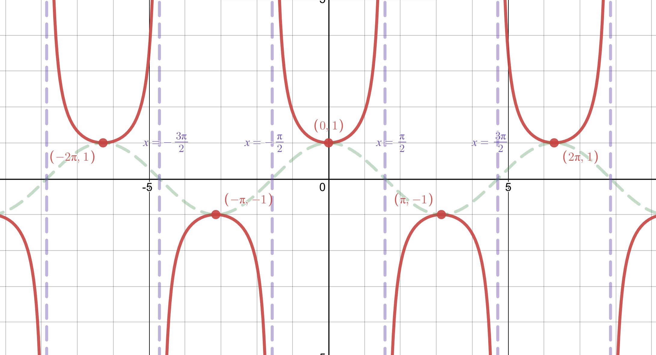
Try playing with the secant graph yourself.
The Cosecant Function
Graphing the cosecant function is extremely similar to graphing the secant function, except we use so we are flipping over the values of sine instead of the values of cosine. Since the sine and cosine graphs look very similar except they are are shifted by , the secant and cosecant graphs will also look very similar but be shifted from one another in the exact same way.
Let’s create the table of famous values for cosecant.
Values of Cosecant in Quadrant I
Values of Cosecant in Quadrant II
Values of Cosecant in Quadrant III
Values of Cosecant in Quadrant IV
Plotting the data in the table along with the expected asymptotes and connecting the points intuitively, we see the graph of the cosecant function.
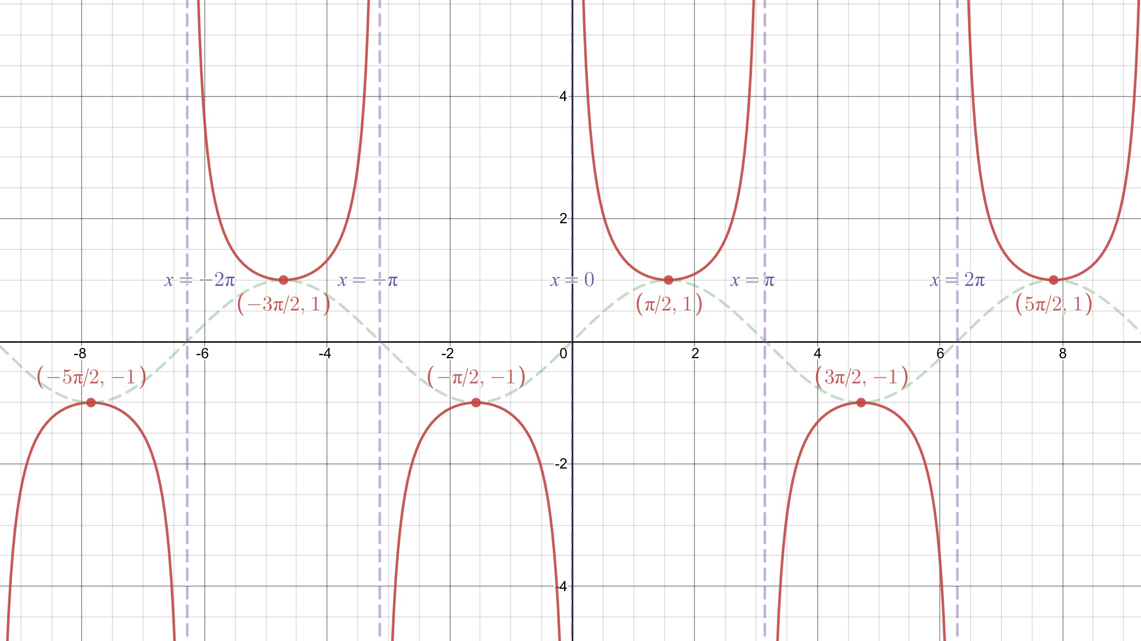
We see from both the table and the graph that the cosecant function has period . We summarize our recent work as follows.
For the function ,
- its domain is the set of all real numbers except where is any whole number;
- its range is the set of all real numbers such that ;
- its period is .
Try playing with the cosecant graph yourself.
The Cotangent Function
Graphing the cotangent function is similar to graphing the secant and cosecant functions, except we use so we are flipping over the values of tangent. Since the tangent graph has a period of , the graph of cotangent will also have a period of . Therefore, we only need to calculate tables of values for the first two quadrants.
Let’s create the table of famous values for cotangent.
Values of Cotangent in Quadrant I
Notice that something unusual happened here. Even though tangent is undefined at , we have that . This is because and so we can define .
Values of Cotangent in Quadrant II
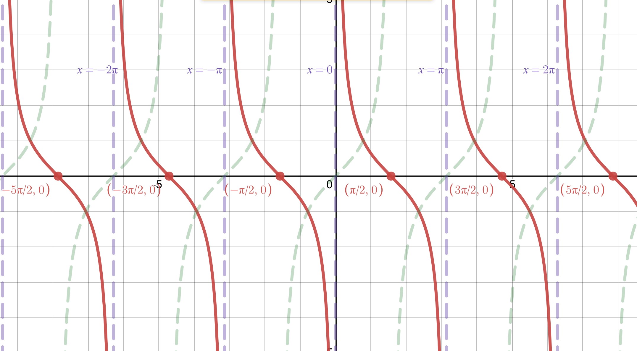
Plotting the data in the table along with the expected asymptotes and connecting the points intuitively, we see the graph of the cotangent function.
For the function ,
- its domain is the set of all real numbers except where is any whole number;
- its range is the set of all real numbers;
- its period is .
Try playing with the cotangent graph yourself.