Introduction
As a review, we go over the list of famous functions from earlier. Then, we move to a discussion of conic sections.
Linear Functions
Recall that the graph of a linear function is a line.


In general, linear functions can be written as where and can be any numbers. We learned that represents the slope, and is the -coordinate of the -intercept. You can play with changing the values of and on the graph using Desmos and see how that changes the line.
Note that a linear function defined by with is odd. If , then is periodic, since it is constant. Furthermore, constant functions are always even.
Additionally, if , then a linear function is one-to-one, and therefore invertible. We summarize this information in the table below.
Note that any real number can be plugged into , so the domain of linear functions is . Unless , we can find a such that , so the range of linear functions with is . If , then the only output of the linear function is , so its range is .
Quadratic Functions
Recall that the graph of a quadratic function is a parabola.


In general, quadratic functions can be written as where , , and can be any numbers. You can play with changing the values of , , and on the graph using Desmos and see how that changes the parabola.
Note that for a quadratic function defined by , if , then is even. In general, quadratic functions are not one-to-one, odd, or periodic, except in cases where , in which we’re actually dealing with a linear function.
Note that any real number can be plugged into , so the domain of quadratic functions is . In Chapter 4, we saw that all quadratic functions have a vertex form , where the vertex is at . If , all points above the vertex, that is are in the range of the quadratic, and if , all points below the vertex, that is are in the range of the quadratic.
We summarize this information in the table below.
Absolute Value Function
Another important type of function is the absolute value function. This is the function that takes all -values and makes them positive. The absolute value function is written as


Notice that the absolute value function is even. Is it one-to-one? The fact that it’s even tells us that it is not, since for all . We summarize this information in the table below.
Note that any real number has an absolute value, so the domain of the absolute value function is . Furthermore, by looking at the graph, we can see that all non-negative numbers are in the range of the absolute value function.
Square Root Function
Another famous function is the square root function,


The square root function is one-to-one. Negative inputs are not valid for the square root function, so it is neither even, odd, nor periodic. We summarize this information in the table below.
Note that only non-negative numbers have square roots, so the domain of the square root function is . Furthermore, by looking at the graph, we can see that all non-negative numbers are in the range of the square root function. Algebraically, we can say that for any non-negative , , so is in the range of the square root function.
Exponential Functions
Another famous function is the exponential growth function,

Here is the mathematical constant known as Euler’s number. .

In general, we can talk about exponential functions of the form where is a positive number not equal to . You can play with changing the values of on the graph using Desmos and see how that changes the graph. Pay particular attention to the difference between and .
Notice that exponential functions are one-to-one, and therefore invertible. However, they are neither even, odd, nor periodic.
Note that the domain of the exponential functions is . Furthermore, by looking at the graph, we can see that all non-negative numbers are in the range of the exponential functions.
We summarize this information in the table below.
Logarithm Functions
Another group of famous functions are logarithms.

In general, we can talk about logarithmic functions of the form where is a positive number not equal to . You can play with changing the values of on the graph using Desmos and see how that changes the graph. Pay particular attention to the difference between and .
Notice that logarithms are neither even, odd, nor periodic. However, they are one-to-one, and therefore invertible. It turns out that the inverse of a logarithm is an exponential function, and vice versa!
Note that since the logarithm is the inverse of the exponential, the domain of the logarithms is the range of the exponentials: . Furthermore, the range of the logarithms is the range of the exponentials: .
We summarize this information in the table below.
Sine
Another important function is the sine function,

This function comes from trigonometry. In the table below we will use another mathematical constant, (“pi” pronounced pie). .

As mentioned earlier, the sine function is odd and periodic with period . Since it is periodic, however, it cannot be one-to-one, since its values repeat.
Note that the domain of the sine function is . Furthermore, by looking at the graph, we can see that its range is .
We summarize this information in the table below.
In general, we can consider . You can play with changing the values of and on the graph using Desmos and see how that changes the graph.
Cosine
A function introduced in Section 3-2 is the cosine function,

As with sine, the cosine function comes from trigonometry. In the table below we will again use .

As mentioned earlier, the cosine function is even and periodic with period . Since it is periodic, however, it cannot be one-to-one, since its values repeat.
Note that the domain of the cosine function is . Furthermore, by looking at the graph, we can see that its range is .
We summarize some information in the table below.
In general, we can consider . You can play with changing the values of and on the graph using Desmos and see how that changes the graph.
Tangent
A function introduced in Section 4-1 is the tangent function,

As mentioned earlier, the tangent function is odd and periodic with period . Since it is periodic, however, it cannot be one-to-one, since its values repeat. Note that the domain of the tangent function is all real numbers except for odd multiples of , since tangent is undefined at those places. Furthermore, by looking at the graph, we can see that its range is . We summarize some information in the table below.
In general, we can consider . You can play with changing the values of and on the graph using Desmos and see how that changes the graph.
Conic Sections
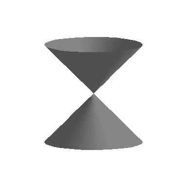
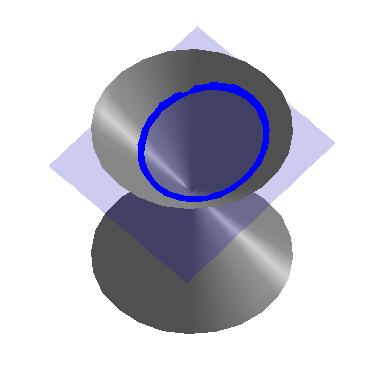
In this section, we study the Conic Sections - literally ‘sections of a cone’. Imagine a double-napped cone as seen below being ‘sliced’ by a plane.
If we slice the cone with a horizontal plane the resulting curve is a circle.
 | 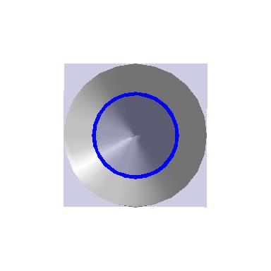 |
Tilting the plane ever so slightly produces an ellipse.
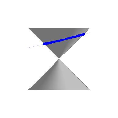 |  |
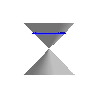
If the plane cuts parallel to the cone, we get a parabola.
 | 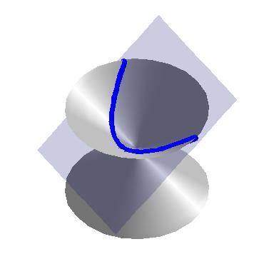 |
If we slice the cone with a vertical plane, we get a hyperbola.
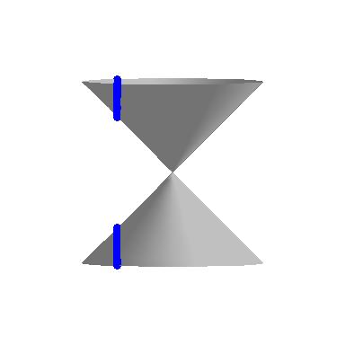 | 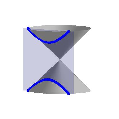 |
For a wonderful animation describing the conics as intersections of planes and cones, see Dr. Louis Talman’s Mathematics Animated Website.
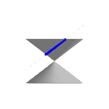
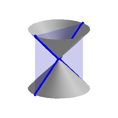
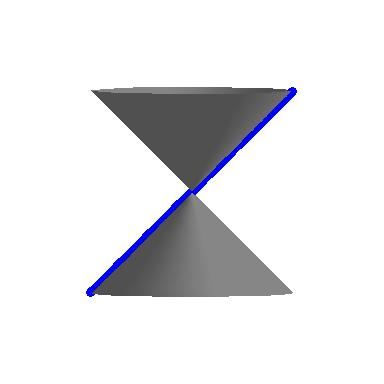
If the slicing plane contains the vertex of the cone, we get the so-called ‘degenerate’ conics: a point, a line, or two intersecting lines.
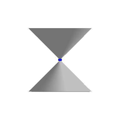 | 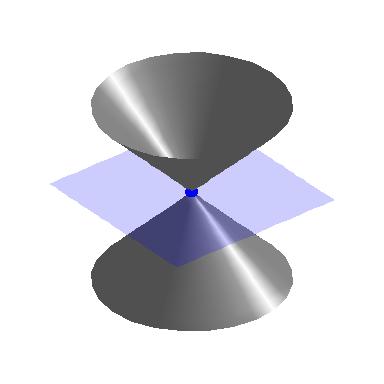 |
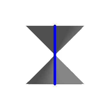 |  |
 | 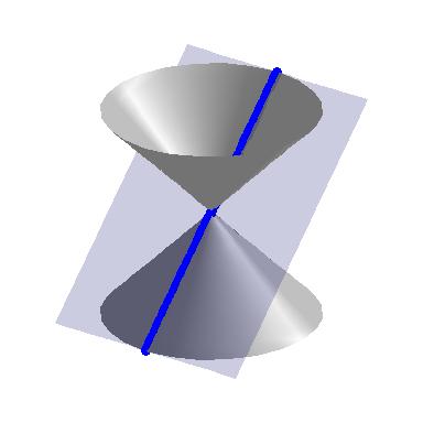 |
We will focus the discussion on the non-degenerate cases: circles, parabolas, ellipses, and hyperbolas, in that order. It’s not necessary to memorize the description of each conic section. We’d just like you to understand that each conic section is the graph of an equation which can be rearranged into a certain standard equation. This standard equation is useful, because it allows us to say something about various geometric properties of the graph. In addition, we will only discuss conic sections centered at the origin.
Circles
Recall from Geometry that a circle can be determined by fixing a point (called the center) and a positive number (called the radius) as follows.

We express this relationship algebraically using the Distance Formula as By squaring both sides of this equation, we get an equivalent equation (since ) which gives us the standard equation of a circle.
This is the first example of a standard equation. If we are given a standard equation of a circle, we can easily find its center and its radius, which is all that we need to be able to draw the circle in the -plane. In other courses, we would spend a lot of time taking an equation, converting it into a standard equation, recognizing it as the standard equation of a conic section, and then using the information provided by the standard equation to graph the relation. For our purposes, we only need to know that this process can be done.
We close this section with the most important circle in all of mathematics: the unit circle.
As you have seen, the unit circle is central to the study of trigonometry.
Parabolas
We know that parabolas are the graphs of quadratic functions. To our surprise and delight, we may also define parabolas in terms of distance.

Each dashed line from the point to a point on the curve has the same length as the dashed line from the point on the curve to the line . The point suggestively labeled is, as you should expect, the vertex. Notice that the focus is not actually a point on the parabola, but only serves to help in its construction.
As with circles, there is a standard equation for parabolas.
If , the parabola opens upwards; if , it opens downwards. The focal length of the parabola is the distance from the focus to the vertex.
Notice that in the standard equation of the parabola above, only one of the variables, , is squared. This is a quick way to distinguish an equation of a parabola from that of a circle because in the equation of a circle, both variables are squared.
Recall from our earlier discussion of inverse functions that interchanging the roles of and results in reflecting the graph across the line . Therefore, if we interchange the roles of and , we can produce ‘horizontal’ parabolas: parabolas which open to the left or to the right. The directrices (plural of ‘directrix’) of such animals would be vertical lines and the focus would either lie to the left or to the right of the vertex, as seen below.

If , the parabola opens to the right; if , it opens to the left.
Ellipses
In the definition of a circle, we fixed a point called the center and considered all of the points which were a fixed distance from that one point. For our next conic section, the ellipse, we fix two distinct points and a distance to use in our definition.
In the figure below, is the distance from to , and is the distance from to . Since is on the ellipse, for some fixed .

We may imagine taking a length of string and anchoring it to two points on a piece of paper. The curve traced out by taking a pencil and moving it so the string is always taut is an ellipse. Notice again that the foci are not actually points on the ellipse, but only serve to help in its construction.
The center of the ellipse is the midpoint of the line segment connecting the two foci. The major axis of the ellipse is the line segment connecting two opposite ends of the ellipse which also contains the center and foci. The minor axis of the ellipse is the line segment connecting two opposite ends of the ellipse which contains the center but is perpendicular to the major axis. The major axis is always the longer of the two segments. The vertices of an ellipse are the points of the ellipse which lie on the major axis. Notice that the center is also the midpoint of the major axis, hence it is the midpoint of the vertices. In pictures we have,

There is also a standard equation for ellipses.
First note that the values and determine how far in the and directions, respectively, one counts from the center to arrive at points on the ellipse. Also take note that if , then we have an ellipse whose major axis is horizontal, and hence, the foci lie to the left and right of the center. In this case, the distance from the center to the focus, , can be found by . If , the roles of the major and minor axes are reversed, and the foci lie above and below the center. In this case, . In either case, is the distance from the center to each focus, and . Finally, it is worth mentioning that if we take the standard equation of a circle and divide both sides by , we get
Notice the similarity between the two equations. Both involve a sum of squares equal to ; the difference is that with a circle, the denominators are the same, and with an ellipse, they are different. If we take a transformational approach, we can consider both equations as shifts and stretches of the unit circle . Replacing with and with causes the usual horizontal and vertical shifts. Replacing with and with causes the usual vertical and horizontal stretches. In other words, it is perfectly fine to think of an ellipse as the deformation of a circle in which the circle is stretched farther in one direction than the other.
Hyperbolas
In the definition of an ellipse, we fixed two points called foci and looked at points whose distances to the foci always added to a constant distance . Those prone to syntactical tinkering may wonder what, if any, curve we’d generate if we replaced added with subtracted. The answer is a hyperbola.

In the figure above:
and
Note that the hyperbola has two parts, called branches. The center of the hyperbola is the midpoint of the line segment connecting the two foci. The transverse axis of the hyperbola is the line segment connecting two opposite ends of the hyperbola which also contains the center and foci. The vertices of a hyperbola are the points of the hyperbola which lie on the transverse axis. In addition, there are lines called asymptotes which the branches of the hyperbola approach for large and values. They serve as guides to the graph. In pictures,

The above hyperbola has center , foci and , and vertices and . The asymptotes are represented by dashed lines.
The conjugate axis of a hyperbola is the line segment through the center which is perpendicular to the transverse axis and has the same length as the line segment through a vertex which connects the asymptotes.
As with all the other conic sections, we have a standard equation for hyperbolas.
If the roles of and were interchanged, then the hyperbola’s branches would open upwards and downwards and we would get a ‘vertical’ hyperbola.
The values of and determine how far in the and directions, respectively, one counts from the center to determine the rectangle through which the asymptotes pass. In both cases, the distance from the center to the foci, , can be found by the formula . Lastly, note that we can quickly distinguish the equation of a hyperbola from that of a circle or ellipse because the hyperbola formula involves a difference of squares where the circle and ellipse formulas both involve the sum of squares.