- How do the three standard transformations (vertical translation, horizontal translation, and vertical scaling) affect the midline, amplitude, range, and period of sine and cosine curves?
- What algebraic transformation results in horizontal stretching or scaling of a function?
- How can we determine a formula involving sine or cosine that models any circular periodic function for which the midline, amplitude, period, and an anchor point are known?
Recall our previous work with transformations, where we studied how the graph of the function defined by is related to the graph of , where , , , and are real numbers with . Because such transformations can shift and stretch a function, we are interested in understanding how we can use transformations of the sine and cosine functions to fit formulas to circular functions.
- a.
- and
- b.
- and
- c.
- and
- d.
- and
- a.
- The graph of has a vertical stretch by 3 and an amplitude of 3. The graph of has a reflection across the -axis with a vertical shrink of and an amplitude of . and both have a midline at and a period of .
- b.
- The graph of has a horizontal shift to the right of . The graph of has a horizontal shift to the left of . and both have a midline at , a period of , and an amplitude of .
- c.
- The graph of has a vertical shift up of and a midline at . The graph of has a vertical shift down of and a midline of . and both have a period of and an amplitude of .
- d.
- The graph of has a vertical stretch by 3, a horizontal shift to the right of ,and a vertical shift up of . has an amplitude of 3 and a midline at . The graph of has a reflection across the -axis with a vertical shrink of , a horizontal shift to the left of , and a vertical shift down of . has an amplitude of and a midline of . and both have a period of .
Note in the exercise above several patterns. Given a function , the amplitude of the function was , and the midline of the function was . In addition, each function above had period , unchanged from the period of . We will see later that this is related to the fact that there were no horizontal stretches or compressions of .
Shifts and vertical stretches of the sine and cosine functions
We know that the standard functions and are circular functions that each have midline , amplitude , period , and range . This suggests the following general principles.
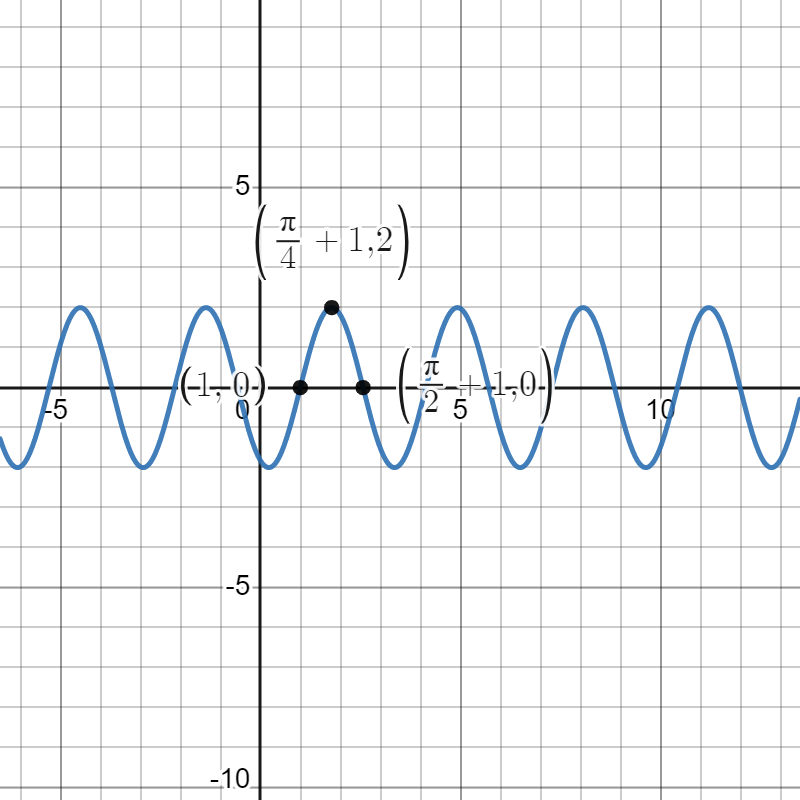
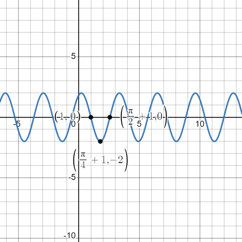
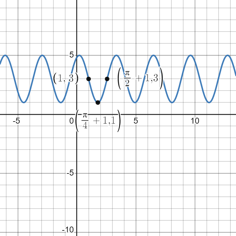
Given real numbers , , and with , the functions each represent a horizontal shift by units to the right, followed by a vertical stretch by units, followed by a vertical shift of units, applied to the parent function ( or , respectively). The resulting circular functions have midline , amplitude , range , and period . In addition, the point lies on the graph of and the point lies on the graph of .
In the figure below, we see how the overall transformation comes from executing a sequence of simpler ones. The original parent function (in red) is first shifted units right to generate the blue graph of . In turn, that graph is then scaled vertically by to generate the orange graph of . Finally, the orange graph is shifted units vertically to result in the final graph of in black.
While the sine and cosine functions extend infinitely in either direction, it’s natural to think of the point as the “starting point” of the cosine function, and similarly the point as the starting point of the sine function. We will refer to the corresponding points and on and as anchor points. Anchor points, along with other information about a circular function’s amplitude, midline, and period help us to determine a formula for a function that fits a given situation.
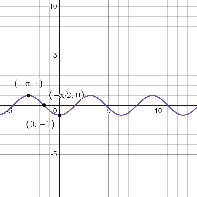
Determine a formula for in the form or . Is it possible to find two different formulas that work?
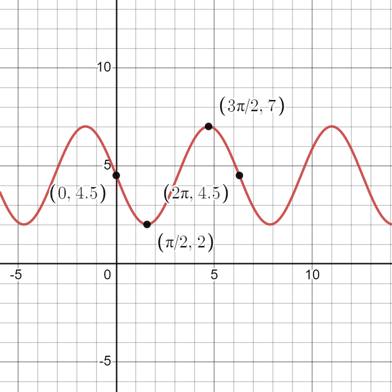
Since the minimum value of is 2 and the maximum value is 7, the midline of must be their midpoint, or . Now we can find the amplitude by finding the distance from the midline to the minimum (or maximum), which would be .
Now we can try to find a formula that uses the sine function. Because the amplitude of is 1, we must stretch by a factor of 2.5 to obtain the correct amplitude of . This results in a transformed function of . Because the midline of is 0, we must shift up by 4.5 to get the midline that we want, resulting in the transformed function . Now has the correct amplitude, midline, and period (unchanged from ). The graph of looks like this:
After some examination, we can see that the only change we need to make to obtain the graph of is to shift units to the left, so that the points and are on the graph of . Therefore, is a formula for in terms of the sine function.
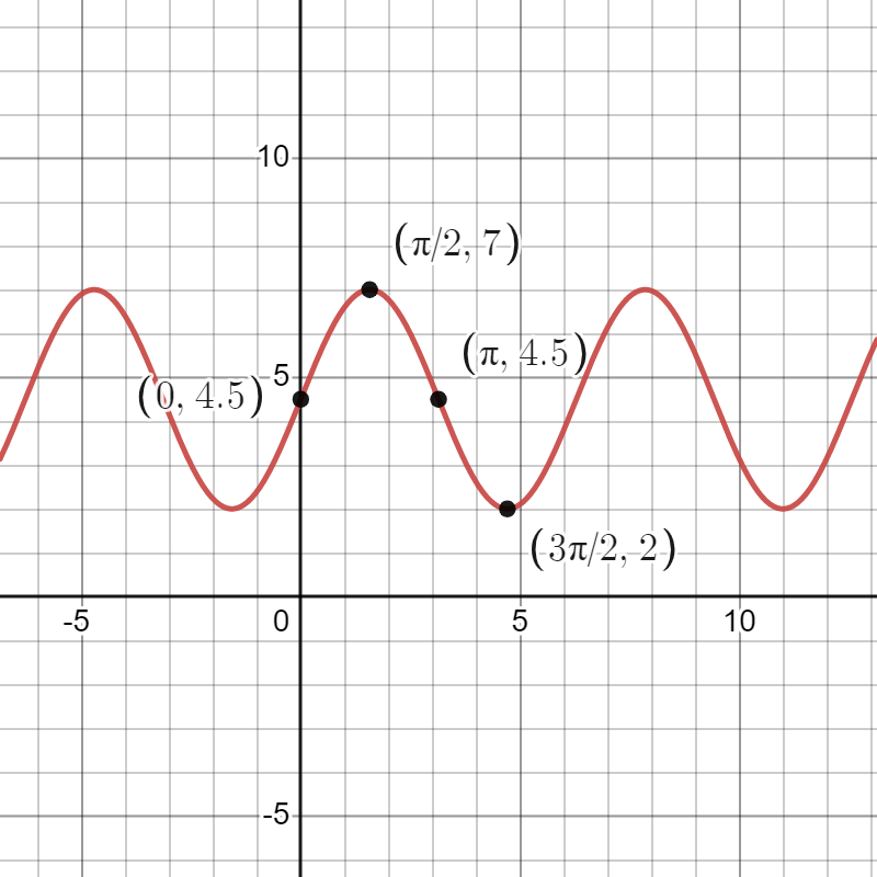
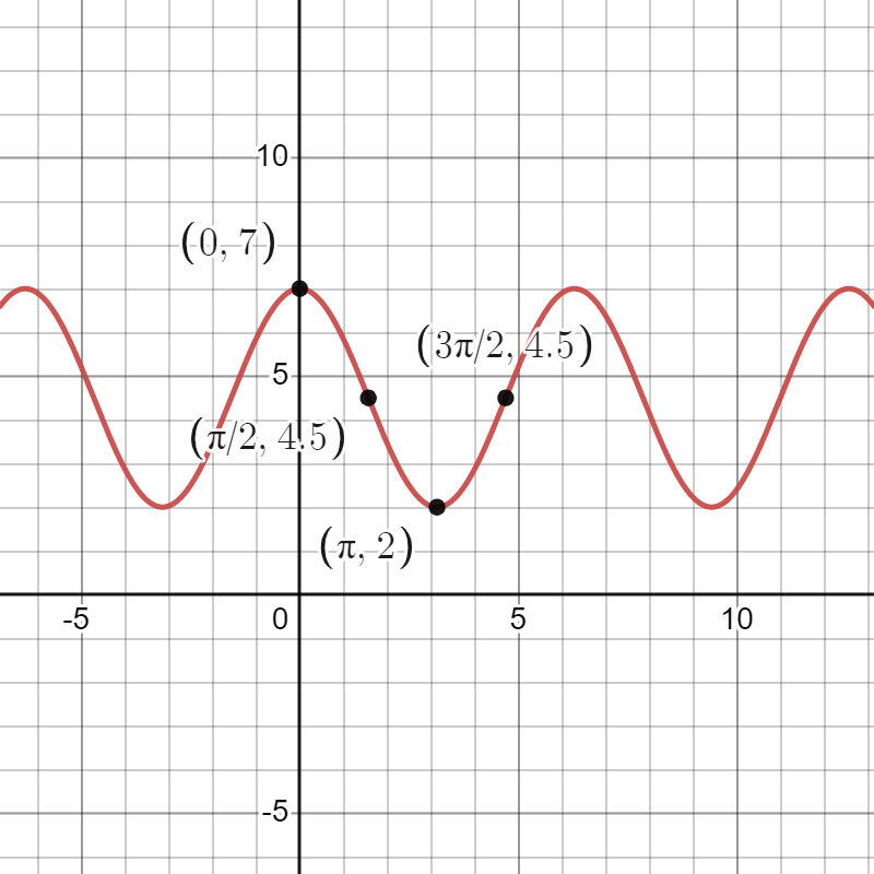
Note that we said that was only a formula for . Let’s try to find a formula using . Since the amplitude of is also 1, we still need to stretch by a factor of 2.5, yielding . Again, since the midline of is 0, we need to shift up by 4.5 units, yielding . The graph of this time looks as follows:
The previous example illustrates a general technique for giving the formula of the graph of a circular function of period with a given midline, amplitude, and -intercept. Say is a circular function with period . If the midline is , the amplitude is , and we know that , then we have a procedure to follow to produce a formula for .
- (a)
- Stretch the graph vertically by a factor of to obtain
- (b)
- Shift the graph vertically up by units to obtain
- (c)
- Find such that
- (d)
- Shift the function horizontally so that the point transforms into .
Note that this procedure can work with as well as . Let’s see an example.
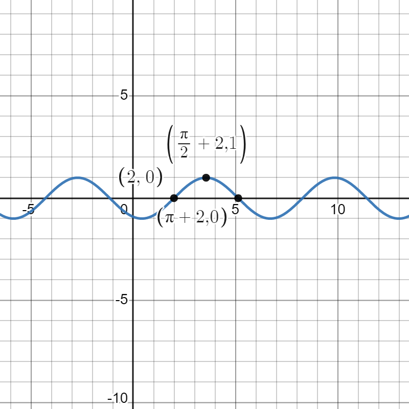
We then proceed using the order of transformations outlined in a previous section. The first transformation to take place is the horizontal shift left by units. That results in the function and moves our points to , , and .
Next, we have a vertical stretch by a factor of 7. This results in the function and moves our points to , , and .
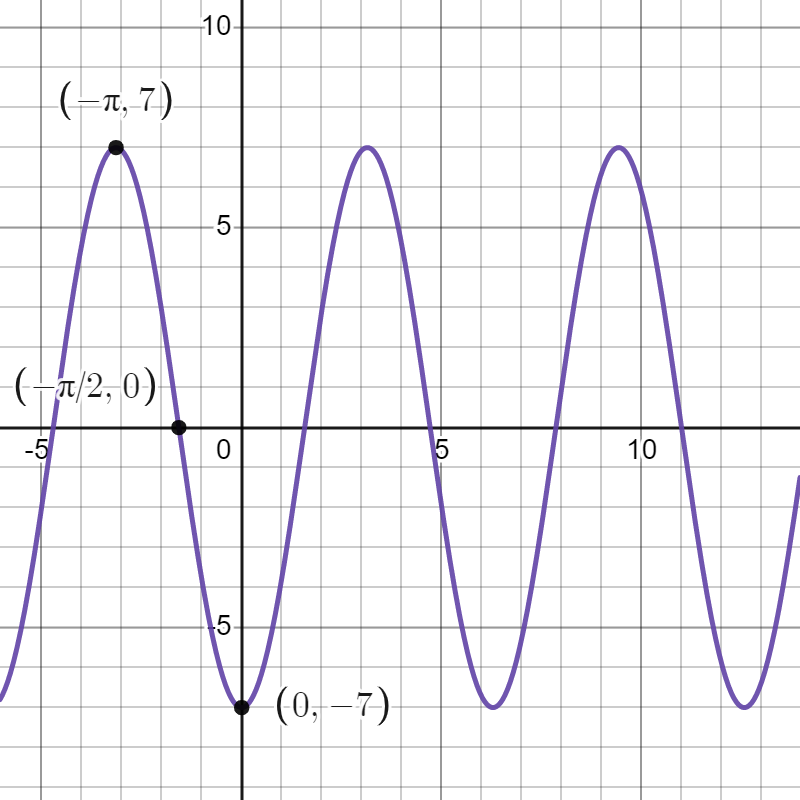
Finally, we shift down by 1 unit. This results in the function and moves our points to , , and .
We can see from the graph that the midline of our function is , and the amplitude is 7. The period can also be read off as . Note that we could have read this information off from the formula, since , , and there is no horizontal stretch or compression.
Horizontal scaling
There is one more very important transformation of a function that we’ve not yet explored in the trigonometric context. Given a function , we want to understand the related function , where is a positive real number. The sine and cosine functions are ideal functions with which to explore these effects; moreover, this transformation is crucial for being able to use the sine and cosine functions to model phenomena that oscillate at different frequencies.
By using a graphing utility such as Desmos, we can explore the effect of the transformation , where .
By experimenting with the slider, we gain an intuitive sense for how the value of affects the graph of in comparision to the graph of . When , we see that the graph of is oscillating twice as fast as the graph of since completes two full cycles over an interval in which completes one full cycle. In contrast, when , the graph of oscillates half as fast as the graph of , as completes only half of one cycle over an interval where completes a full one.
We can also understand this from the perspective of function composition. To evaluate , at a given value of , we first multiply the input by a factor of , and then evaluate the function at the result. An important observation is that This tells us that the point lies on the graph of since an input of in results in the value . At the same time, the point lies on the graph of . Thus we see that the correlation between points on the graphs of and (where ) is We can therefore think of the transformation as achieving the output values of twice as fast as the original function does. Analogously, the transformation will achieve the output values of only half as quickly as the original function.
Recall that given a function and a real number , the transformed function is a horizontal stretch of the graph of . Every point on the graph of gets stretched horizontally to the corresponding point on the graph of . If , the graph of is a stretch of away from the -axis by a factor of ; if , the graph of is a compression of toward the -axis by a factor of . The only point on the graph of that is unchanged by the transformation is .
Circular functions with different periods
Because the circumference of the unit circle is , the sine and cosine functions each have period . Of course, as we think about using transformations of the sine and cosine functions to model different phenomena, it is apparent that we will need to generate functions with different periods than . For instance, if a ferris wheel makes one revolution every minutes, we’d want the period of the function that models the height of one car as a function of time to be . Horizontal scaling of functions enables us to generate circular functions with any period we desire.
We begin by considering two basic examples. First, let and . We know from our most recent work that this transformation results in a horizontal compression of the graph of by a factor of toward the -axis. If we plot the two functions on the same axes, it becomes apparent how this transformation affects the period of .
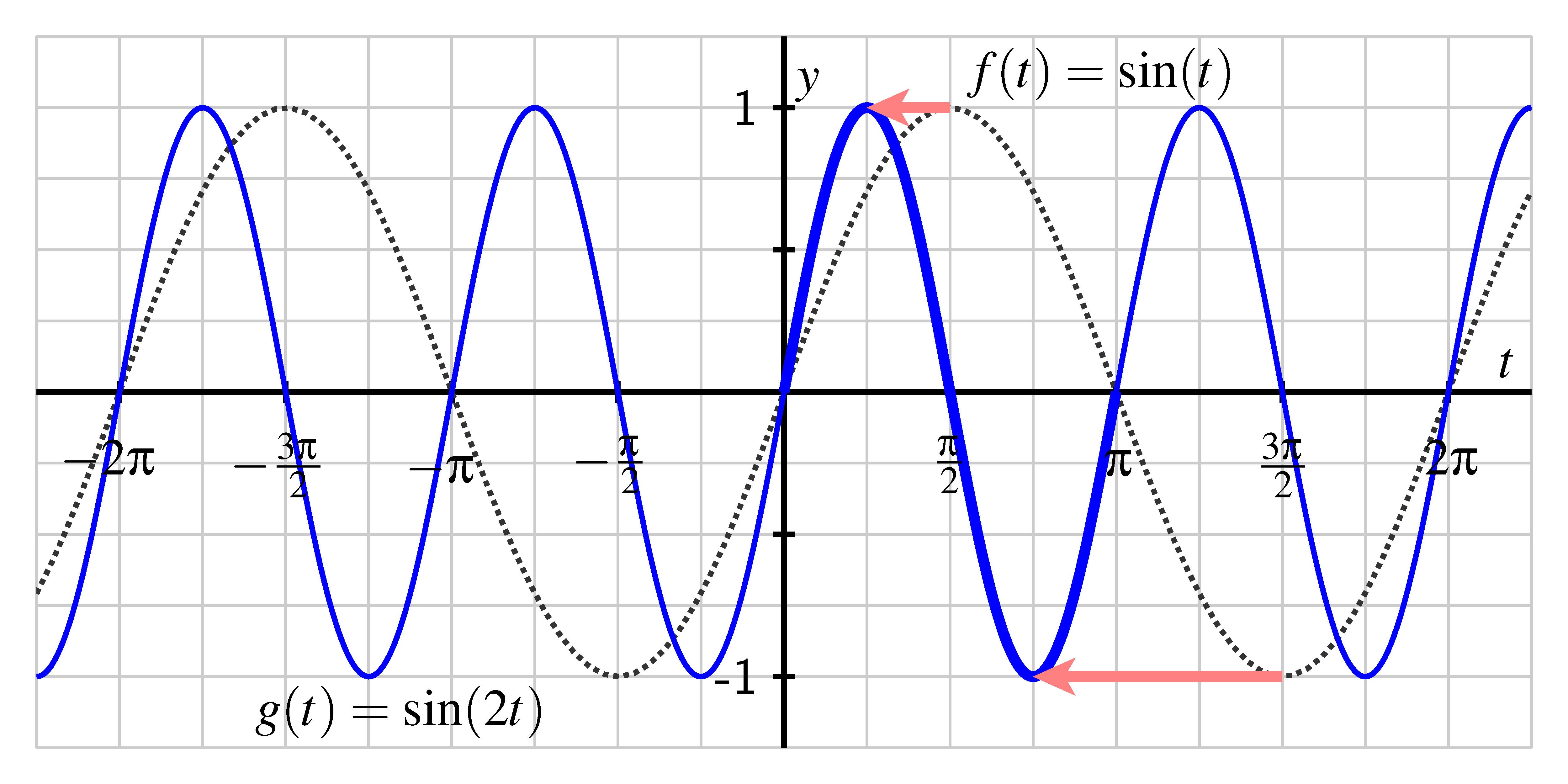
From the graph, we see that oscillates twice as frequently as , and that completes a full cycle on the interval , which is half the length of the period of . Thus, the “” in causes the period of to be as long; specifially, the period of is .
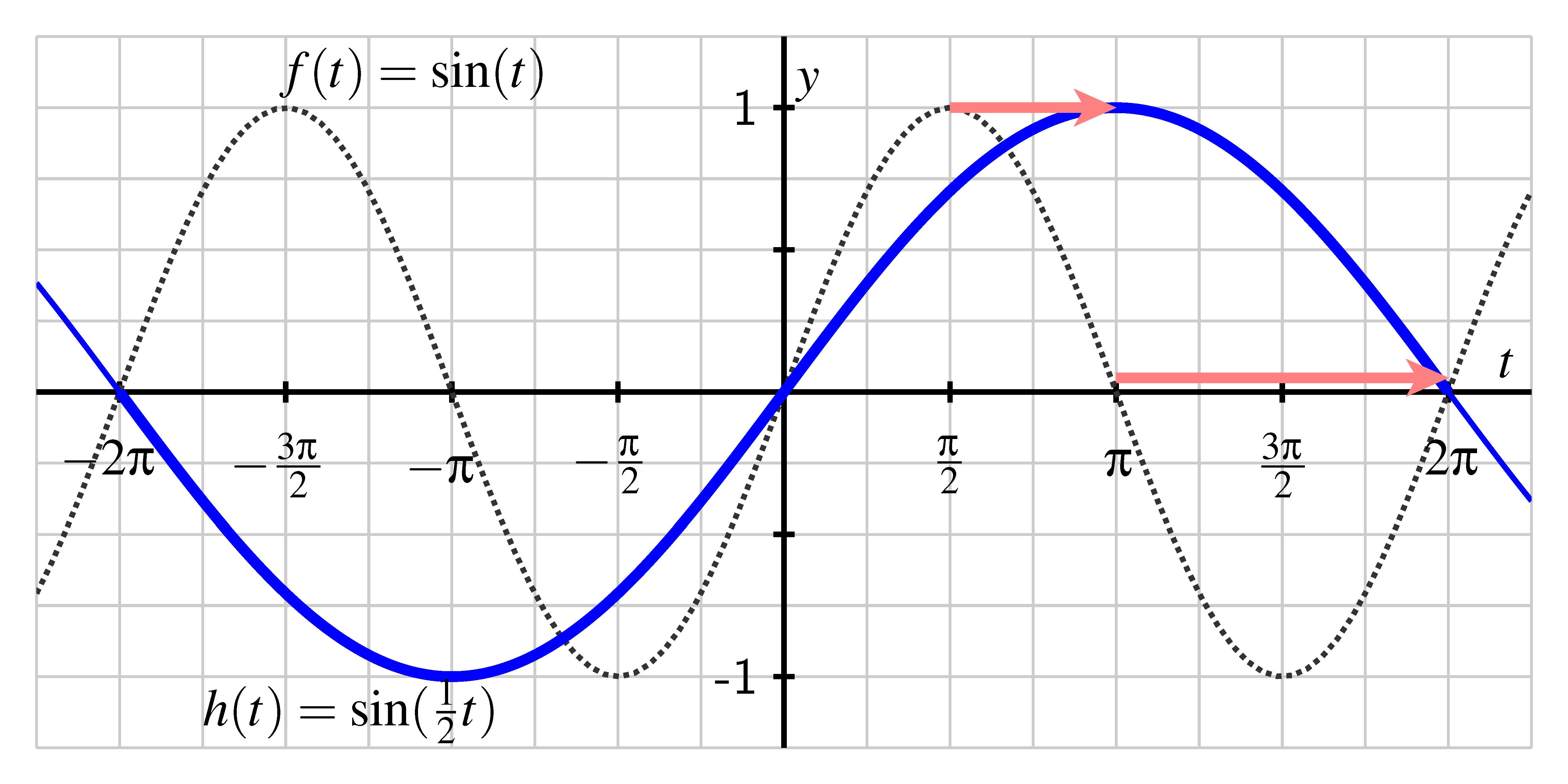
On the other hand, if we let , the transformed graph is stretched away from the -axis by a factor of . This has the effect of doubling the period of , so that the period of is , as seen in the previous figure.
Our observations generalize for any positive constant . In the case where , we saw that the period of is , whereas in the case where , the period of is . Identical reasoning holds if we are instead working with the cosine function. In general, we can say the following.
For any constant , the period of the functions and is
Thus, if we know the -value from the given function, we can deduce the period. If instead we know the desired period, we can determine by the rule .
Given real numbers , , , and with and , the functions each represent a horizontal stretch or compression by a factor of , followed by a vertical stretch by units, followed by a vertical shift of units, applied to the parent function ( or , respectively). They then contain a horizontal shift to the right by units. The resulting circular functions have midline , amplitude , range , and period . In addition, the point lies on the graph of and the point lies on the graph of .
- a.
- b.
- c.
- d.
- e.
- a.
- has a period of , an amplitude of and a midline of .
The range of is . - b.
- has a period of , an amplitude of and a midline of .
The range of is . - c.
- has a period of , an amplitude of and a midline of .
The range of is . - d.
- has a period of , an amplitude of and a midline of .
The range of is .
There is a horizontal shift of to the right. - e.
- has a period of , an amplitude of and a midline of .
The range of is .
There is a horizontal shift of to the right. This is because we have to factor out the 3 inside the parentheses: .
You might wonder why we’ve chosen to use the formula with the parentheses instead of without the parentheses. In the former formula, we save the horizontal shift until the end, but in the latter, we do the horizontal shift before anything else. The reason we prefer the former is that the midline, amplitude, and period of a function are easy to plug into the formula, and plugging these in results in a formula of the form . We can then find the horizontal shift we need to apply to the graph of to obtain .
State the midline, amplitude, range, and an anchor point for the function, and hence determine a formula for in the form or . Show your work and thinking, and use Desmos appropriately to check that your formula generates the desired behavior.
Since we started with the cosine function, we know that the maximum of is 4, and occurs at . Since we want , we need to shift our graph to the right by 1.25 units. This means . We can then check that by plugging into our function.
Let’s now pay some attention to the choice between sine and cosine. Note that since the midline is and the amplitude is , the maximum of our function is . This means that the condition that tells us where the maximum should be. We have a very easy location for the maximum of cosine: , so we’ll choose to use cosine here. Note that choosing sine isn’t incorrect, just more difficult.
Plugging our values into the equation, we have . The maximum for cosine occurs at , as stated above, but we want the maximum to occur at , so we’ll shift the graph of 8 units to the right. This gives us .
Here, the amplitude is 3, the midline is , and the period is . Using the sine function as a parent function, this gives us . Note that , and we want our function to have , so we need to shift the graph of to the right by 1 unit. This gives us .
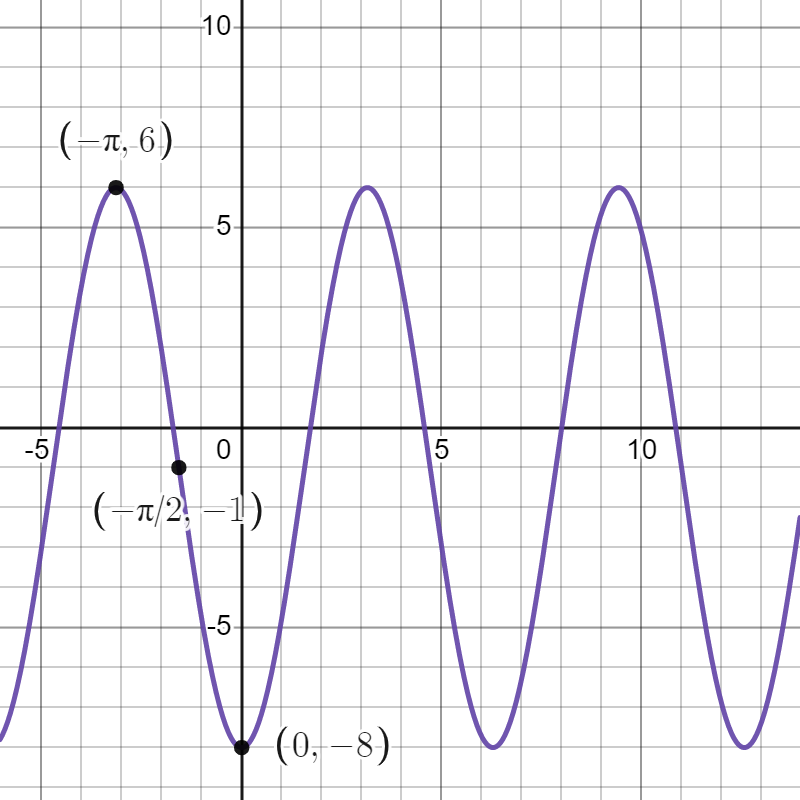
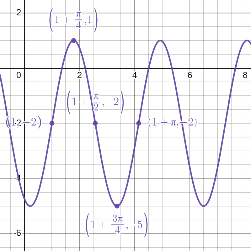
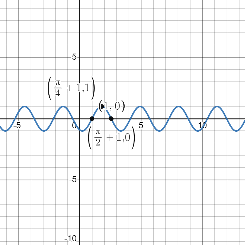
With this change, we can see that our first transformation is a shift right by 2 units, yielding . This transforms our points into , , and . We can see a graph of below.
Our next transformation in the order is a horizontal compression by a factor of 2, yielding . This transforms our points into , , and . We can see a graph of below.
Our next transformation is a vertical stretch by a factor of 2, yielding . This transforms our points into , , and . We can see a graph of below.
Our next transformation is a reflection across the -axis, yielding . This transforms our points into , , and . We can see a graph of below.
Our final transformation is a shift up by 3 units, yielding . This transforms our points into , , and . We can see a graph of below.
The midline of is 3, the amplitude is 2, and the period is . This is all readable from the graph, but also from the formula for , since , , and .
You may have noticed that the last example involved a reflection, a transformation we have not talked about in the context of circular functions. This is because reflections of circular functions turn out to be obtainable by shifts, so when we’re given graphical information and asked to reconstruct the formula for a function, we don’t need to use reflections. Reflections may show up when we are given a formula and asked to provide a graph. But we already have lots of practice producing graphs in this situation and can draw on this prior experience with transformations.
- Given real numbers , , and with , the functions each represent a horizontal shift by units to the right, followed by a vertical stretch by units, followed by a vertical shift of units, applied to the parent function ( or , respectively). The resulting circular functions have midline , amplitude , range , and period . In addition, the anchor point lies on the graph of and the anchor point lies on the graph of .
- Given a function and a constant , the algebraic transformation results in horizontal scaling of by a factor of . In particular, when , the graph of is compressed toward the -axis by a factor of to create the graph of , while when , the graph of is stretched away from the -axis by a factor of to create the graph of .
- Given any circular periodic function for which the midline, amplitude, period, and an anchor point are known, we can find a corresponding formula for the function of the form Each of these functions has period midline , amplitude , and period . The point lies on and the point lies on .