- a.
- Recall that the circumference, , of a circle is connected to the circle’s radius, , by the formula . What is the radius of the ferris wheel? How high is the highest point on the ferris wheel?
- b.
- How high is the cab after it has traveled of the circumference of the circle?
- c.
- How much distance along the circle has the cab traversed at the moment it first reaches a height of meters?
- d.
- Can be thought of as a function of ? Why or why not?
- e.
- Can be thought of as a function of ? Why or why not?
- f.
- Why do you think the curve shown above has the shape that it does? Write several sentences to explain.
Motivating Questions
- How does a point traversing a circle naturally generate a function?
- What are some important properties that characterize a function generated by a point traversing a circle?
Certain naturally occurring phenomena eventually repeat themselves, especially when the phenomenon is somehow connected to a circle. You may recall from when we first studied periodic functions that we considered the case of taking a ride on a ferris wheel. We considered your height, , above the ground and how your height changed in tandem with the distance, , that you have traveled around the wheel. We saw a snapshot of this situation, which is available as a full animation at http://gvsu.edu/s/0Dt.
A snapshot of the motion of a cab moving around a ferris wheel. Reprinted with permission from Illuminations by the National Council of Teachers of Mathematics. All rights reserved.
Because we have two quantities changing in tandem, it is natural to wonder if it is possible to represent one as a function of the other.
In the context of the ferris wheel
pictured above, assume that the height, , of the moving point (the cab in which you
are riding), and the distance, , that the point has traveled around the circumference
of the ferris wheel are both measured in meters. Further, assume that the
circumference of the ferris wheel is meters. In addition, suppose that after getting in
your cab at the lowest point on the wheel, you traverse the full circle several
times.
Circular Functions
The natural phenomenon of a point moving around a circle leads to interesting relationships. Let’s consider a point traversing a circle of circumference and examine how the point’s height, , changes as the distance traversed, , changes. Note particularly that each time the point traverses of the circumference of the circle, it travels a distance of units, as seen below where each noted point lies additional units along the circle beyond the preceding one.
Note that we know the exact heights of certain points. Since the circle has circumference , we know that and therefore . Hence, the point where (located of the way along the circle) is at a height of . Doubling this value, the point where has height . Other heights, such as those that correspond to and (identified on the figure by the green line segments) are not obvious from the circle’s radius, but can be estimated from the grid in the graph above as (for ) and (for ). Using all of these observations along with the symmetry of the circle, we can determine the other entries in the table below.
Data for height, , as a function of distance traversed, .
Moreover, if we now let the point continue traversing the circle, we observe that the -values will increase accordingly, but the -values will repeat according to the already-established pattern, resulting in the data in the table below.
Additional data for height, , as a function of distance traversed, .
It is apparent that each point on the circle corresponds to one and only one height, and thus we can view the height of a point as a function of the distance the point has traversed around the circle, say . Using the data from the two tables and connecting the points in an intuitive way, we get the graph shown below.
The height, , of a point traversing a circle of radius as a function of distance, , traversed around the circle.
The function we have been discussing is an example of what we will call a circular function. Indeed, it is apparent that if we:
- take any circle in the plane,
- choose a starting location for a point on the circle,
- let the point traverse the circle continuously,
- and track the height of the point as it traverses the circle,
the height of the point is a function of distance traversed and the resulting graph will have the same basic shape as the curve shown in the graph above. It also turns out that if we track the location of the -coordinate of the point on the circle, the -coordinate is also a function of distance traversed and its curve has a similar shape to the graph of the height of the point (the -coordinate). Both of these functions are circular functions because they are generated by motion around a circle.
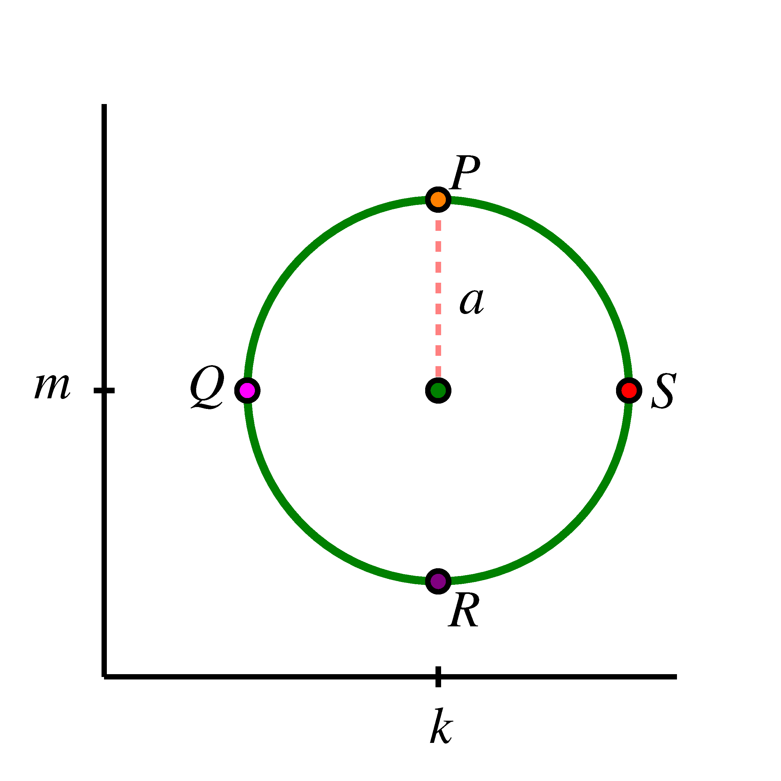
Consider the circle pictured below that is centered at the point and that has
circumference . Assume that we track the -coordinate (that is, the height, ) of a
point that is traversing the circle counterclockwise and that it starts at as
pictured.
- a.
- How far along the circle is the point from ? Why?
- b.
- Label the subsequent points in the figure , , as we move counterclockwise around the circle. What are the exact coordinates of ? of ? Why?
- c.
- Determine the coordinates of the remaining points on the circle (exactly where possible, otherwise approximately) and hence complete the entries in the table below that track the height, , of the point traversing the circle as a function of distance traveled, .
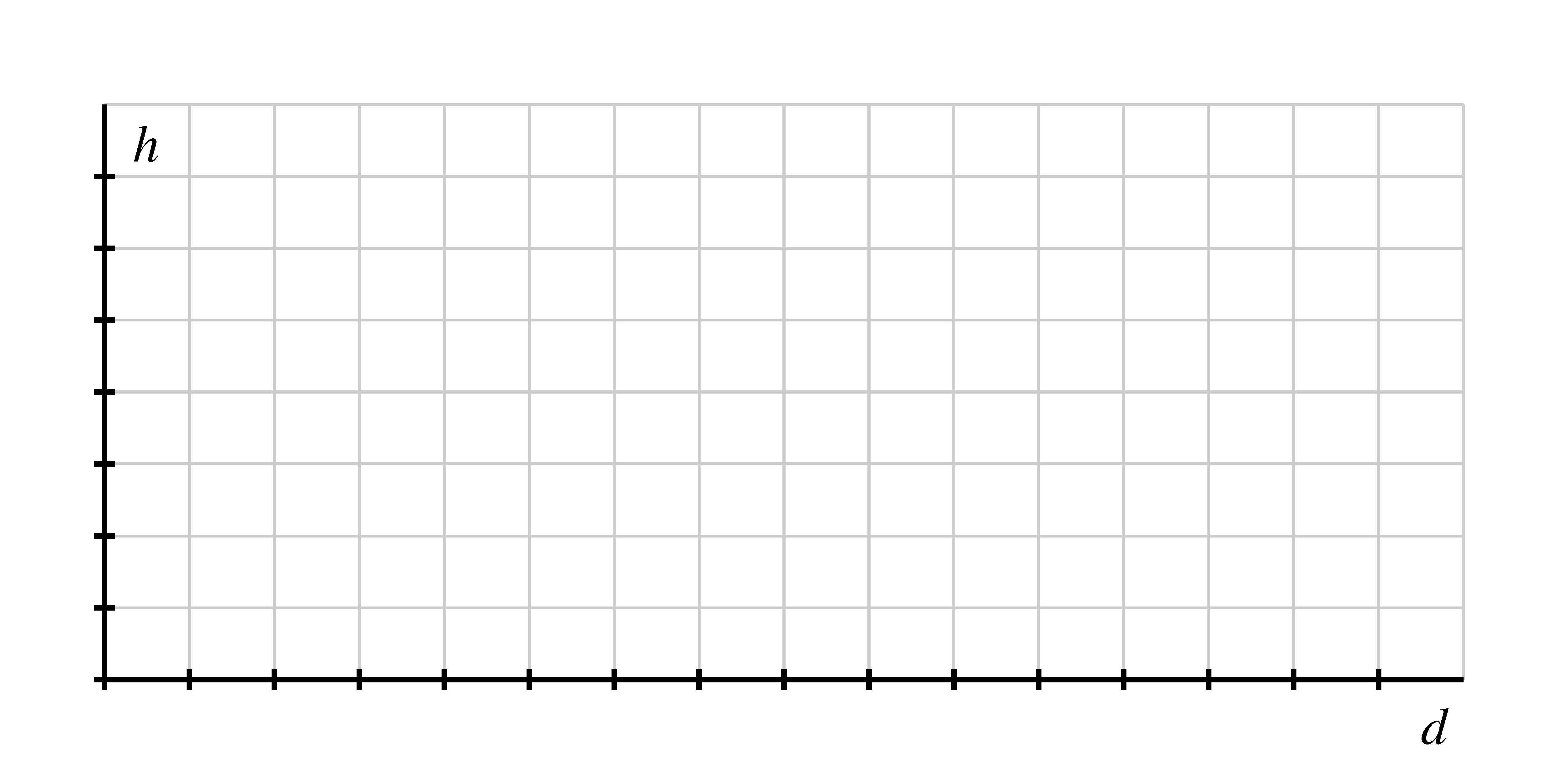
- d.
- By plotting the points in the table and connecting them in an intuitive way,
sketch a graph of as a function of on the axes provided over the interval .
Clearly label the scale of your axes and the coordinates of several important
points on the curve.
- e.
- What is similar about your graph in comparison to the one in we created at the beginning of this section? What is different?
- f.
- What will be the value of when ? How about when ?
Properties of Circular Functions
Every circular function has several important features that are connected to the circle that defines the function. For the discussion that follows, we focus on circular functions that result from tracking the -coordinate of a point traversing counterclockwise a circle of radius centered at the point . Further, we will denote the circumference of the circle by the letter .
We assume that the point traversing the circle starts at in the graph of the circle above. Its height is initially , and then its height decreases to as we traverse to . Continuing, the point’s height falls to at , and then rises back to at , and eventually back up to at the top of the circle. If we plot these heights continuously as a function of distance, , traversed around the circle, we get the curve shown below.
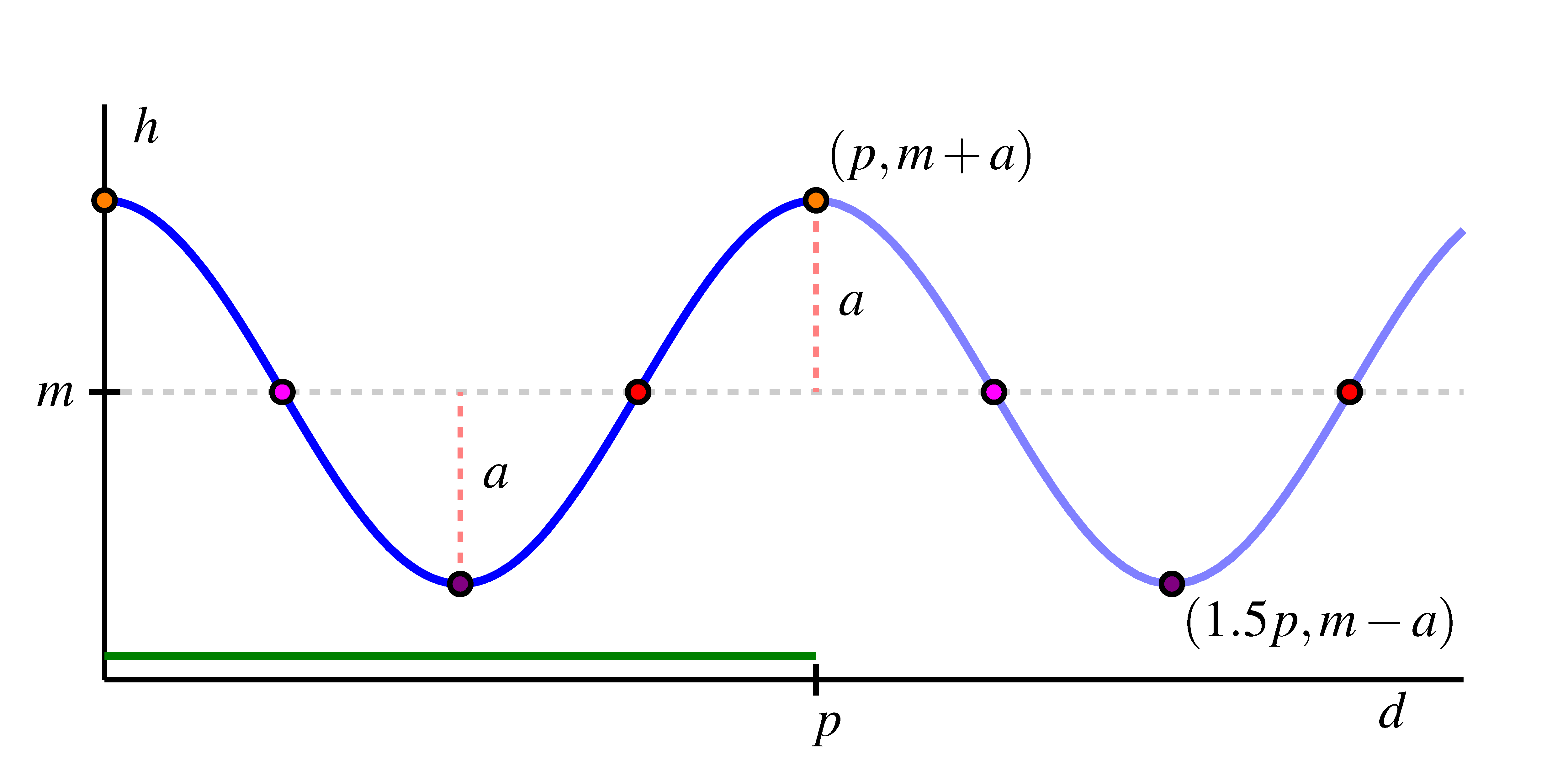
This curve has several important features for which we introduce important terminology.
The midline of a circular function is the horizontal line for which half the curve lies
above the line and half the curve lies below. If the circular function results from
tracking the -coordinate of a point traversing a circle, corresponds to the -coordinate
of the center of the circle. In addition, the amplitude of a circular function is the
maximum deviation of the curve from the midline. Note particularly that the value of
the amplitude, , corresponds to the radius of the circle that generates the
curve.
Because we can traverse the circle in either direction and for as far as we wish, the domain of any circular function is the set of all real numbers. From our observations about the midline and amplitude, it follows that the range of a circular function with midline and amplitude is the interval .
This graph is an example of a periodic function. Recall the definition of a periodic function.
Let be a function whose domain and codomain are each the set of all real numbers.
We say that is periodic provided that there exists a real number such that for
every possible choice of . The smallest value for which for every choice of is called
the period of .
For a circular function, the period is always the circumference of the circle that generates the curve. In the graph of the function above, we see how the curve has completed one full cycle of behavior every units, regardless of where we start on the curve.
Circular functions arise as models for important phenomena in the world around us, such as in a harmonic oscillator. Consider a mass attached to a spring where the mass sits on a frictionless surface. After setting the mass in motion by stretching or compressing the spring, the mass will oscillate indefinitely back and forth, and its distance from a fixed point on the surface turns out to be given by a circular function.
The Average Rate of Change of a Circular Function
Just as there are important trends in the values of a circular function, there are also interesting patterns in the average rate of change of the function. These patterns are closely tied to the geometry of the circle.
For the next part of our discussion, we consider a circle of radius centered at , and consider a point that travels a distance counterclockwise around the circle with its starting point viewed as . We use this circle to generate the circular function that tracks the height of the point at the moment the point has traversed units around the circle from . Let’s consider the average rate of change of on several intervals that are connected to certain fractions of the circumference.
Remembering that is a function of distance traversed along the circle, it follows that the average rate of change of on any interval of distance between two points and on the circle is given by
where both quantities are measured from point to point .First, we consider points , , and where results from traversing of the circumference from , and of the circumference from . In particular, we note that the distance along the circle from to is the same as the distance along the circle from to , and thus . At the same time, it is apparent from the geometry of the circle that the change in height from to is greater than the change in height from to , so . Thus, we can say that
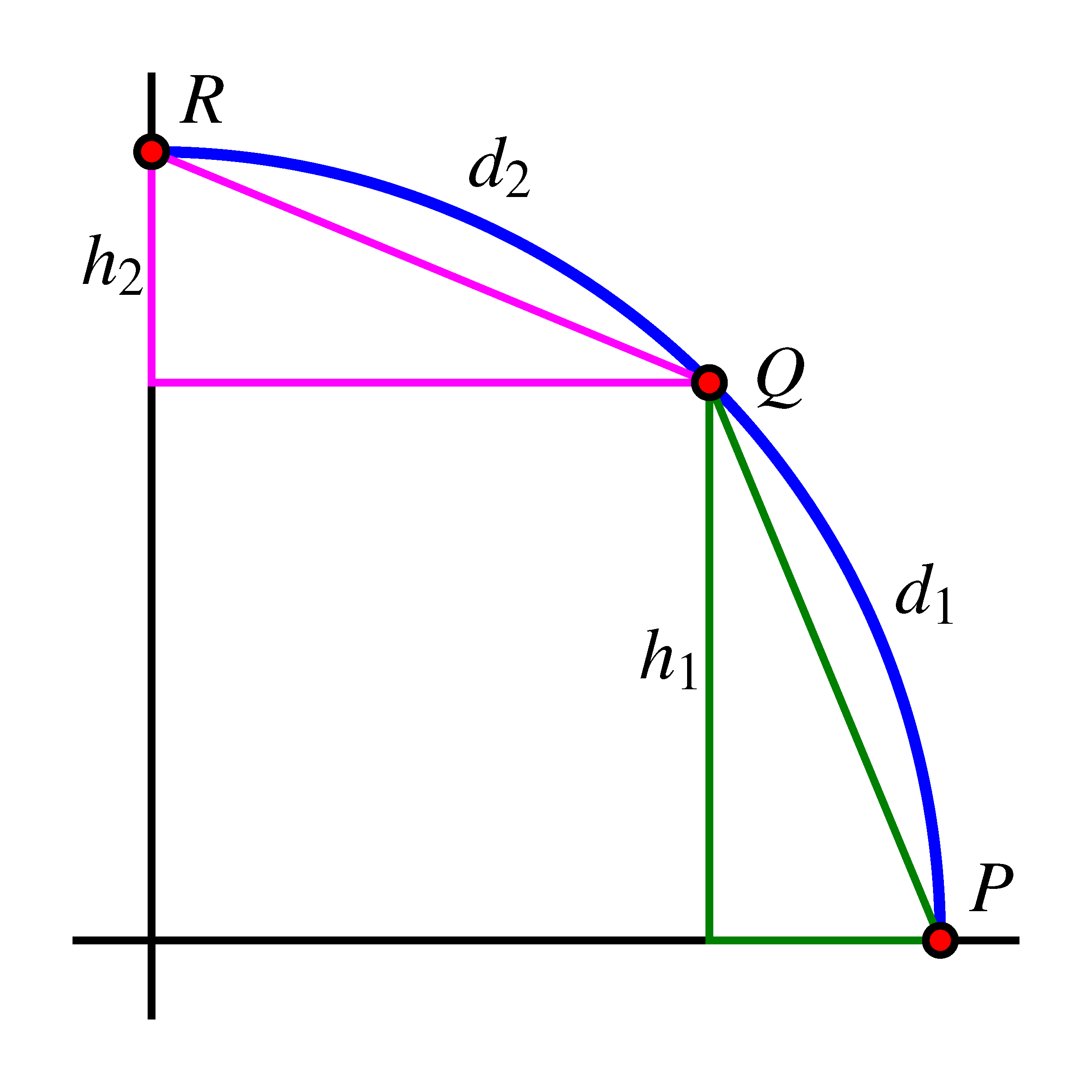
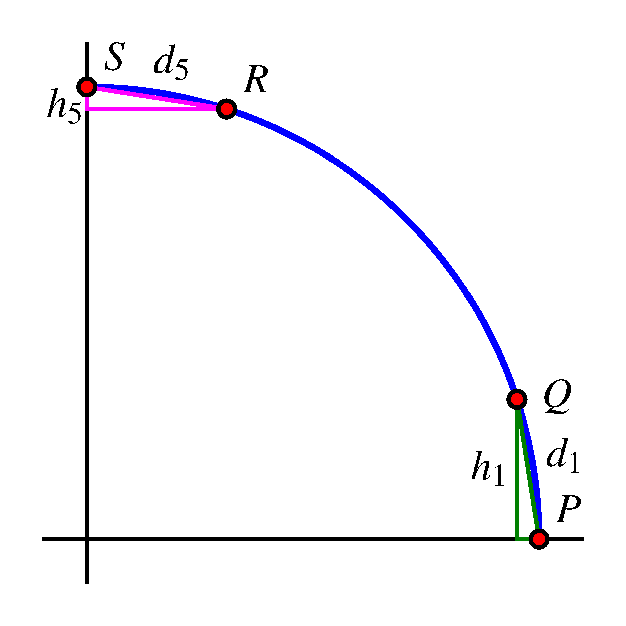
The differences in certain average rates of change appear to become more extreme if we consider shorter arcs along the circle. Next we consider traveling of the circumference along the circle. In the graph below, points and lie of the circumference apart, as do and , so here . In this situation, it is the case that for the same reasons as above, but we can say even more. From the green triangle, we see that (while ), so that . At the same time, in the magenta triangle in the figure we see that is very small, especially in comparison to , and thus . Hence, in this graph,
This information tells us that a circular function appears to change most rapidly for points near its midline and to change least rapidly for points near its highest and lowest values.
We can study the average rate of change not only on the circle itself, but also on a generic circular function graph, and thus make conclusions about where the function is increasing, decreasing, concave up, and concave down.
- When a point traverses a circle, a corresponding function can be generated by tracking the height of the point as it moves around the circle, where height is viewed as a function of distance traveled around the circle. We call such a function a circular function.
- Circular functions have several standard features. The function has a midline that is the line for which half the points on the curve lie above the line and half the points on the curve lie below. A circular function’s amplitude is the maximum deviation of the function value from the midline; the amplitude corresponds to the radius of the circle that generates the function. Circular functions also repeat themselves, and we call the smallest value of for which for all the period of the function. The period of a circular function corresponds to the circumference of the circle that generates the function.
- Non-constant linear functions are either always increasing or always decreasing; quadratic functions are either always concave up or always concave down. Circular functions are sometimes increasing and sometimes decreasing, plus sometimes concave up and sometimes concave down. These behaviors are closely tied to the geometry of the circle.