Introduction
In this section, we will review our earlier discussion about function transformations. In addition, we’ll explore what happens when multiple function transformations occur.
Review of Single Transformations
The following table gives the formulas and descriptions of all the function transformations we learned about. If is the parent function, then the formula in the left column gives the function that corresponds to the transformation of the graph given in the middle column. The right column gives the new location of the point on the graph of .
Putting it Together
Transformations may be performed one after another. If the transformations include stretches, shrinks, or reflections, the order in which the transformations are performed may make a difference. In those cases, be sure to pay particular attention to the order.
- (a)
- The graph of undergoes the following transformations, in order. Find the
equation of the graph that results.
- a horizontal shift 2 units to the right
- a vertical stretch by a factor of 3
- a vertical shift 5 units up
- (b)
- Apply the transformations above in the opposite order and find the equation of the graph that results.
- (a)
- We will use to denote the parent function and to denote the intermediate
functions. Applying the transformations in order we have
- (b)
- Applying the transformations in the opposite order we have
This shows that changing the order in which the transformations are applied may end up changing the resulting function.
The previous example shows how to construct the formula of a function given a sequence of transformations. One might wonder how to find the transformations applied to a parent function’s graph given a complicated formula. That is, if we know a formula , can we reconstruct the sequence of transformations? There are two parts to this: finding the transformations and finding the order of those transformations. The following example gives some of the reasoning behind the process.
Now we have to think about what transformations are being applied to the graph . We can see from the table in the previous section that based on the changes made to the formula, there are
- a horizontal compression by a factor of 2 and
- a horizontal shift 7 units to the left
Note that this is not necessarily the order in which these transformations occur, but an unordered list of them.
It remains for us to find the order in which these transformations were applied to produce the function . It’s a good rule of thumb to start with the transformations closer to the variable , since those are applied to the function first. Let’s try starting with the horizontal compression by a factor of 2. Applying this transformation to yields , since a horizontal compression adds a factor to the variable in the previous function. This seems to be a good start. Next, let’s take care of the horizontal shift by 7 units to the left. Applying this transformation to yields , since shifting 7 to the left adds 7 to the variable in the previous function. Note that since it adds 7 only to the , we have to use parentheses here. However, we’ve gotten off track: , which is not what we wanted to appear inside the absolute value symbols. Let’s try the other order.
This time, begin with the horizontal shift 7 units to the left. Applying this to the parent function yields . Then, move on to the horizontal compression by a factor of 2. Applying this transformation to yields , since according to the table, we multiply only the variable by 2 for this transformation.
This tells us that the correct order for our transformations is
- (a)
- a horizontal shift 7 units to the left and
- (b)
- a horizontal compression by a factor of 2
Let’s see how this fits into a more complicated example.
Now we have to think about what transformations are being applied to the graph . We can see from the table in the previous section that based on the changes made to the formula, there are
- a vertical stretch by a factor of 3,
- a horizontal compression by a factor of 2,
- a horizontal shift 7 units to the left, and
- a vertical shift 2 units down.
Note that this is not necessarily the order in which these transformations occur, but an unordered list of them.
As in the previous example, we begin with the horizontal shift 7 units to the left. Applying this to the parent function yields . Then, move on to the horizontal compression by a factor of 2. Applying this transformation to yields , since according to the table, we multiply only the variable by 2 for this transformation. Next, let’s try taking care of the vertical stretch by a factor of 3. Applying this transformation to gives us , since vertical stretches correspond to multiplying the entire previous function by the factor. Last, we can incorporate the vertical shift 2 units down. Since that corresponds to subtracting 2 from the previous function , we obtain , which is exactly the function we wanted to reconstruct.
This tells us that the correct order for our transformations is
- (a)
- a horizontal shift 7 units to the left,
- (b)
- a horizontal compression by a factor of 2,
- (c)
- a vertical stretch by a factor of 3, and
- (d)
- a vertical shift 2 units down.
Note that if we applied transformations 3 and 4 in a different order, we would have obtained a different function.
Given a function , note that we can apply the same reasoning to to find the order of the transformations applied to the graph of :
- (a)
- horizontal shift,
- (b)
- horizontal stretch or compression,
- (c)
- vertical stretch or compression, and
- (d)
- vertical shift.
One might wonder where reflections fit into all this. Let’s see with another example.
Let’s see what happens if we do the reflections after the stretches or compressions, but before the vertical shift. Following our order, we first shift left by units to obtain , then stretch horizontally by a factor of 3 to obtain , then compress vertically by a factor of 2 to obtain . Flipping vertically puts a minus sign on the outside of the function, giving us . Next, flipping horizontally puts a minus sign on the , giving us . Finally, shifting up by 1 gives us , which is what we wanted in the end.
Note that we could have done the horizontal reflection before the vertical reflection and achieved the same result. Therefore, as long as you do the reflections after the stretches or compressions, it doesn’t matter which order each reflection comes in.
We can summarize all this information as follows. Given a function , the graph of can be found using the following transformations in order:
- (a)
- horizontal shifts given by ,
- (b)
- horizontal stretches or compressions given by ,
- (c)
- vertical stretches or compressions given by ,
- (d)
- reflections given by the sign of and , and
- (e)
- vertical shifts given by .
Note that this is not the only order you can use to graph transformations of functions. This is just one order that works every time, provided you start with a function of the form .
- (a)
- a horizontal shift right by 5 units,
- (b)
- a horizontal compression by a factor of 3,
- (c)
- a vertical compression by a factor of 2,
- (d)
- a reflection across the -axis, and
- (e)
- a vertical shift up by 1 unit.
To graph , we’ll start with the graph of , and by keeping track of the transformations of a few points, , , and , we’ll draw the graph after applying each transformation. To start with, here’s the graph of .
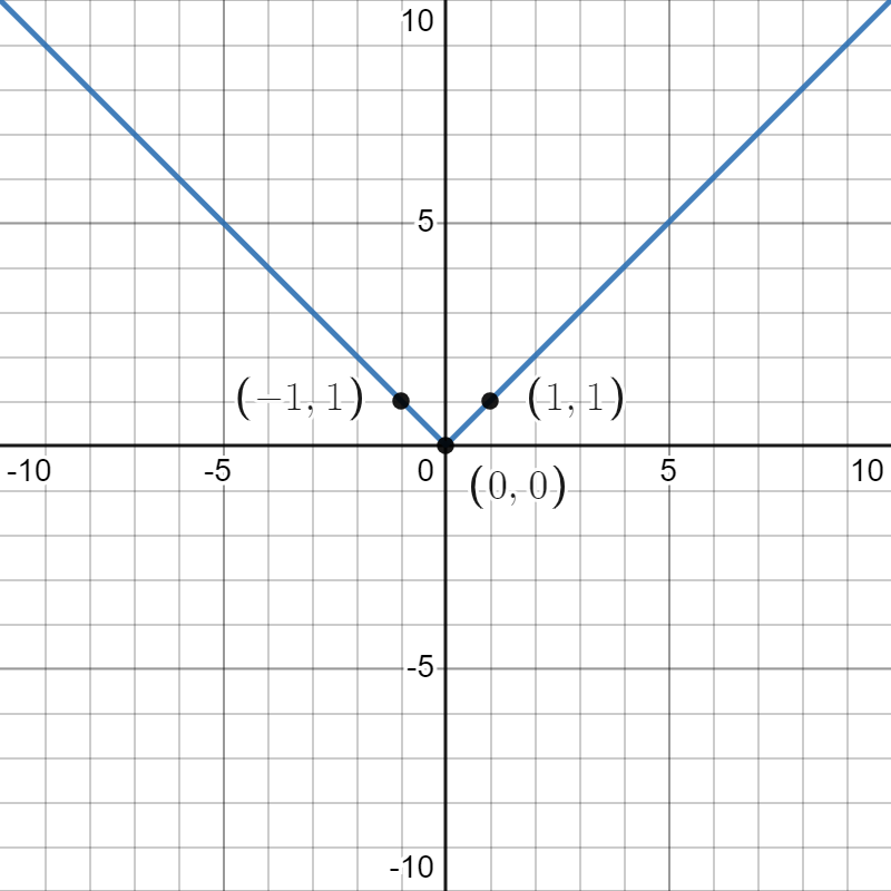
After horizontally shifting right by 5 units, our points are , , and and the graph of looks like this:
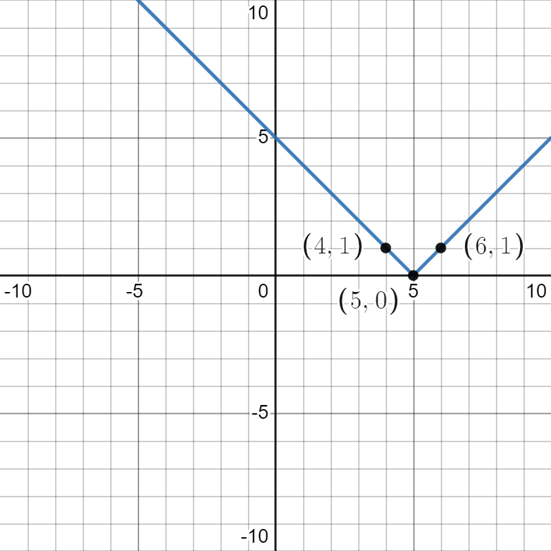
Compressing horizontally by a factor of 3 gives us , and our points are , , and :
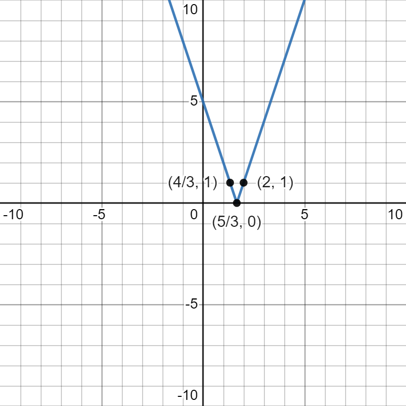
Vertically compressing by a factor of 2 gives us the points , , and and the function :
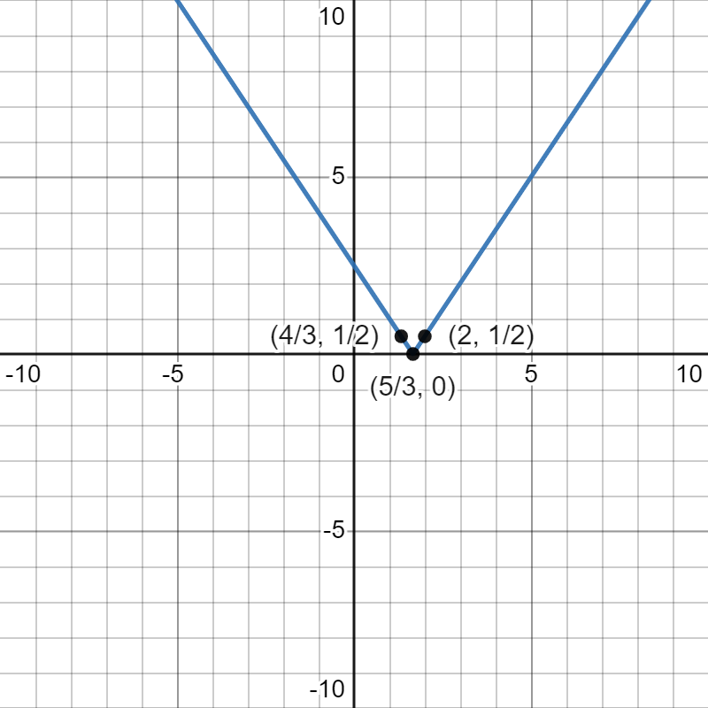
Reflecting across the -axis gives us the points , , and and the function :
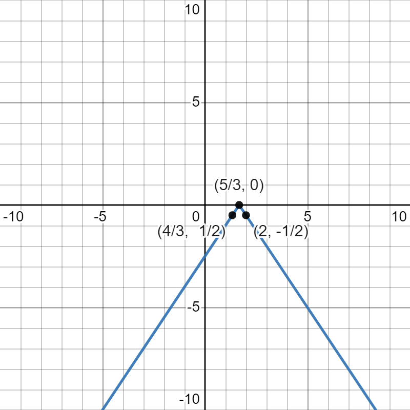
Finally, vertically shifting up by 1 gives us the points , , and and the function :
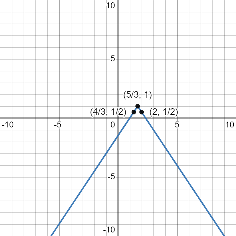
This last graph is our final result. While graphing each step along the way may seem like an awful lot of work, it is often easier than trying to work with multiple transformations at once in your head.
Below is a link to a Desmos graph containing for a function where you can adjust the values of , , , and to see how they affect the graph. The function in the link below is the formula for a half-circle, but don’t worry too much about where it came from.