- a.
- Compute the value of
- b.
- What are the units on the quantity ? What is the meaning of this number in the context of the rising/falling ball?
- c.
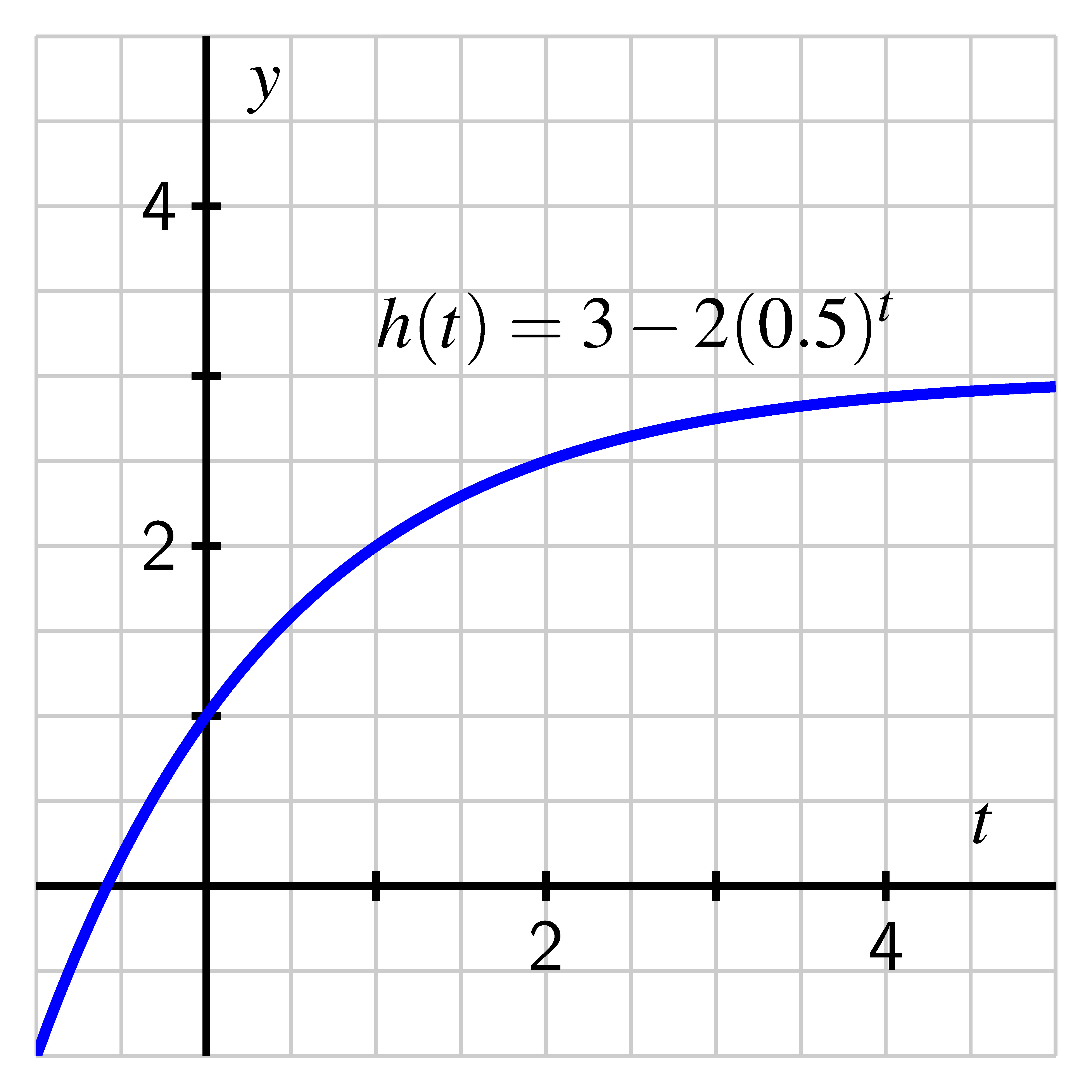
- In Desmos, plot the function along with the points and . Make a copy of your
plot on the axes below, labeling key points as well as the scale on
your axes. What is the domain of the model? The range? Why?
- d.
- Work by hand to find the equation of the line through the points and . Write the line in the form and plot the line in Desmos, as well as on the axes above.
- e.
- What is a geometric interpretation of the value in light of your work in the preceding questions?
- f.
- How do your answers in the preceding questions change if we instead consider the interval ? ? ?
Motivating Questions
- What do we mean by the average rate of change of a function on an interval?
- What does the average rate of change of a function measure? How do we interpret its meaning in context?
- How is the average rate of change of a function connected to a line that passes through two points on the curve?
Given a function that models a certain phenomenon, it’s natural to ask such questions as “how is the function changing on a given interval” or “on which interval is the function changing more rapidly?” The concept of average rate of change enables us to make these questions more mathematically precise. Initially, we will focus on the average rate of change of an object moving along a straight-line path.
First, let’s define some notation for the intervals we will be referring to in this section and going forward.
represents the values of such that . We call this the closed interval from to .
represents the values of such that . We call this the open interval from to .
Notice that the major difference between these intervals is that and are included in
the closed interval but not in the open interval.
For a function that tells the location of a moving object along a straight path at time , we define the average rate of change of between and to be the quantity
Note particularly that the average rate of change of between and is measuring the change in position divided by the change in time. Let the height function for a ball tossed vertically be given by , where is measured
in seconds and is measured in feet above the ground.
Defining and interpreting the average rate of change of a function
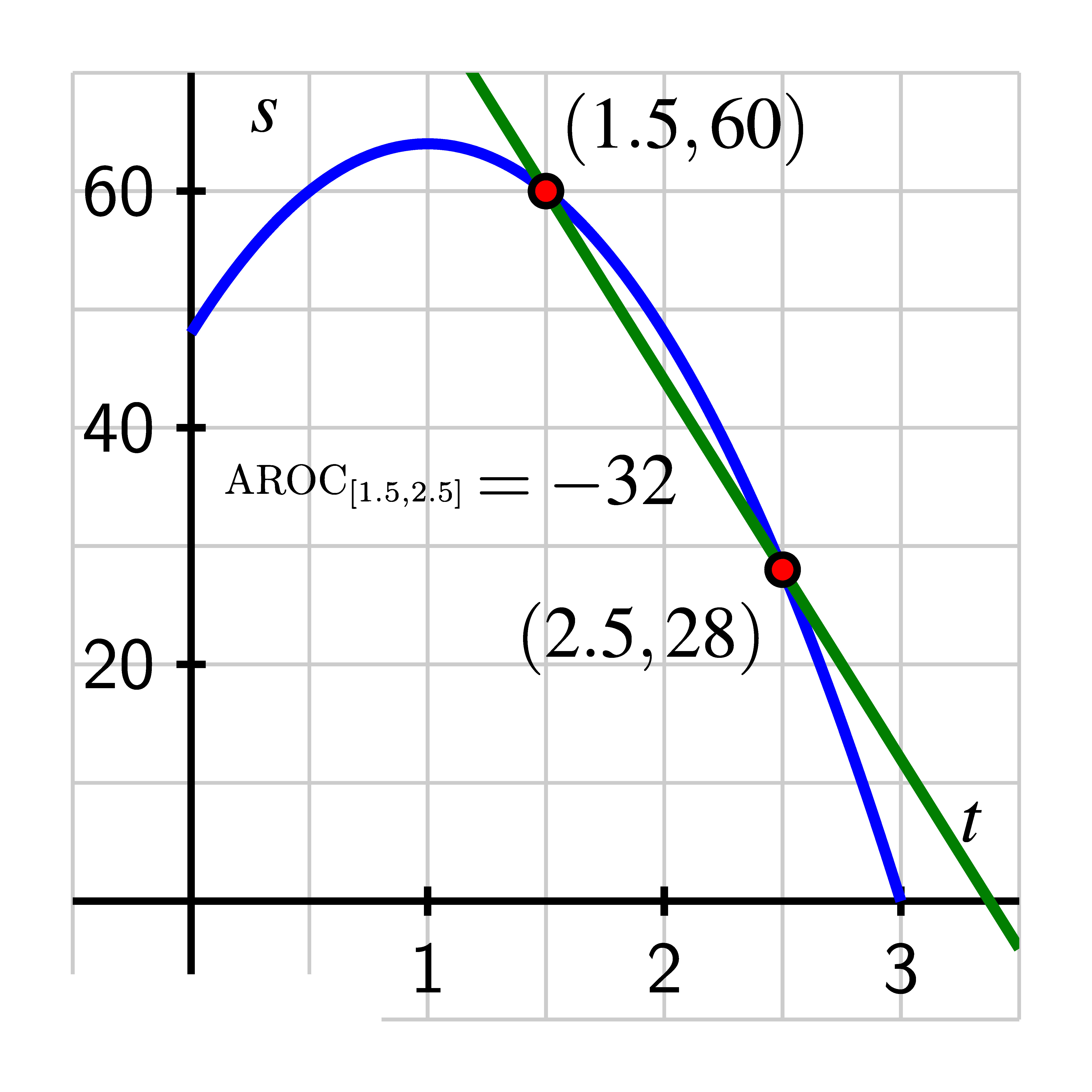
In the context of a function that measures height or position of a moving object at a given time, the meaning of the average rate of change of the function on a given interval is the average velocity of the moving object because it is the ratio of change in position to change in time. For example, in the exploration above, the units on are “feet per second” since the units on the numerator are “feet” and on the denominator “seconds”. Morever, is numerically the same value as the slope of the line that connects the two corresponding points on the graph of the position function, as seen below. The fact that the average rate of change is negative in this example indicates that the ball is falling.
While the average rate of change of a position function tells us the moving object’s average velocity, in other contexts, the average rate of change of a function can be similarly defined and has a related interpretation. We make the following formal definition.
In every situation, the units on the average rate of change help us interpret its meaning, and those units are always “units of output per unit of input.” Moreover, the average rate of change of on always corresponds to the slope of the line between the points and . Before we explore this concept further, we note that this line has a special name, it is the secant line to the graph.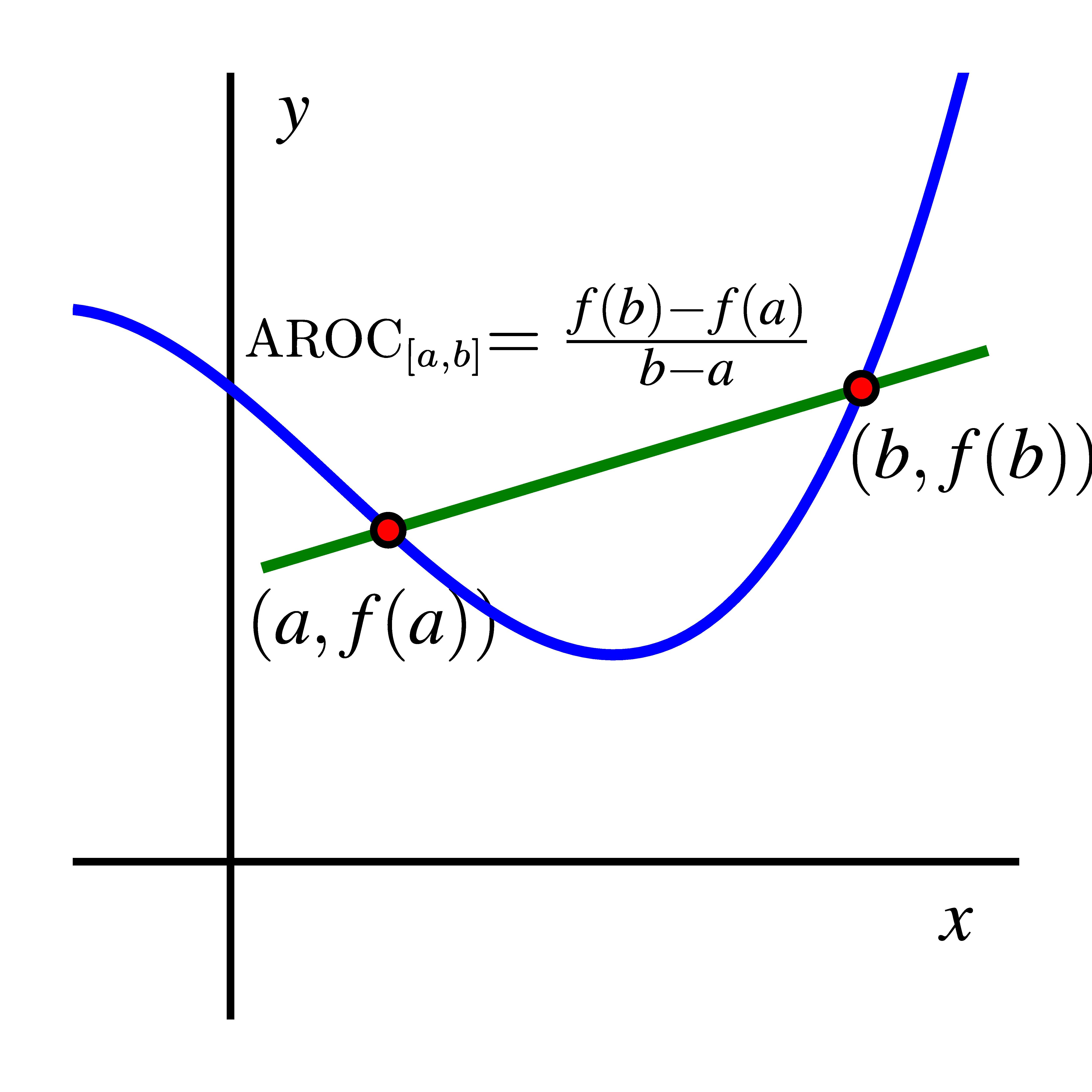
Definition: Consider a function . A line passing through two points and ,
with , in the graph of , is called a secant line to the graph. The slope of
a secant line is the average rate of change of the function on the interval
.
According to the US census, the populations of Kent and Ottawa Counties (Grand
Rapids is in Kent, Allendale in Ottawa) from 1960 to 2010 measured in -year
intervals are given in the following tables.
Kent County Population data
Ottawa County Population data
Let represent the population of Kent County in year and the population of Ottawa County in year Y.
- a.
- Compute for both and .
- b.
- What are the units on each of the quantities you computed in (a.)?
- c.
- Write a careful sentence that explains the meaning of the average rate of change of the Ottawa county population on the time interval . Your sentence should begin something like “In an average year between 1990 and 2010, the population of Ottawa County was ”
- d.
- Which county had a greater average rate of change during the time interval ? Were there any intervals in which one of the counties had a negative average rate of change?
- e.
- Using the given data, what do you predict will be the population of Ottawa County in 2018? Why?
The average rate of change of a function on an interval gives us an excellent way to describe how the function behaves, on average. For instance, if we compute for Kent County, we find that
which tells us that in an average year from 1970 to 2000, the population of Kent County increased by about people. Said differently, we could also say that from 1970 to 2000, Kent County was growing at an average rate of people per year. These ideas also afford the opportunity to make comparisons over time. Since we can not only say that the county’s population increased by about in an average year between 1990 and 2000, but also that the population was growing faster from 1990 to 2000 than it did from 1970 to 2000.Finally, we can even use the average rate of change of a function to predict future behavior. Since the population was changing on average by people per year from 1990 to 2000, we can estimate that the population in 2002 is
How average rate of change indicates function trends
We have already seen that it is natural to use words such as “increasing” and “decreasing” to describe a function’s behavior. For instance, for the tennis ball whose height is modeled by , we computed that , which indicates that on the interval , the tennis ball’s height is decreasing at an average rate of feet per second. Similarly, for the population of Kent County, since , we know that on the interval the population is increasing at an average rate of people per year.
We make the following formal definitions to clarify what it means to say that a function is increasing or decreasing.
Let be a function defined on an interval (that is, on the set of all for which ). We
say that is increasing on provided that the function is always rising as we move
from left to right. That is, for any and in , if , then .
Similarly, we say that is decreasing on provided that the function is always falling as we move from left to right. That is, for any and in , if , then .
Similarly, we say that is decreasing on provided that the function is always falling as we move from left to right. That is, for any and in , if , then .
If a function is increasing, its average rate of change will be positive. If a function is decreasing, its average rate of change will be negative. However the reverse doesn’t necessarily hold true. If we compute the average rate of change of a function on an interval, we can decide if the function is increasing or decreasing on average on the interval, but it takes more work1 to decide if the function is increasing or decreasing always on the interval.
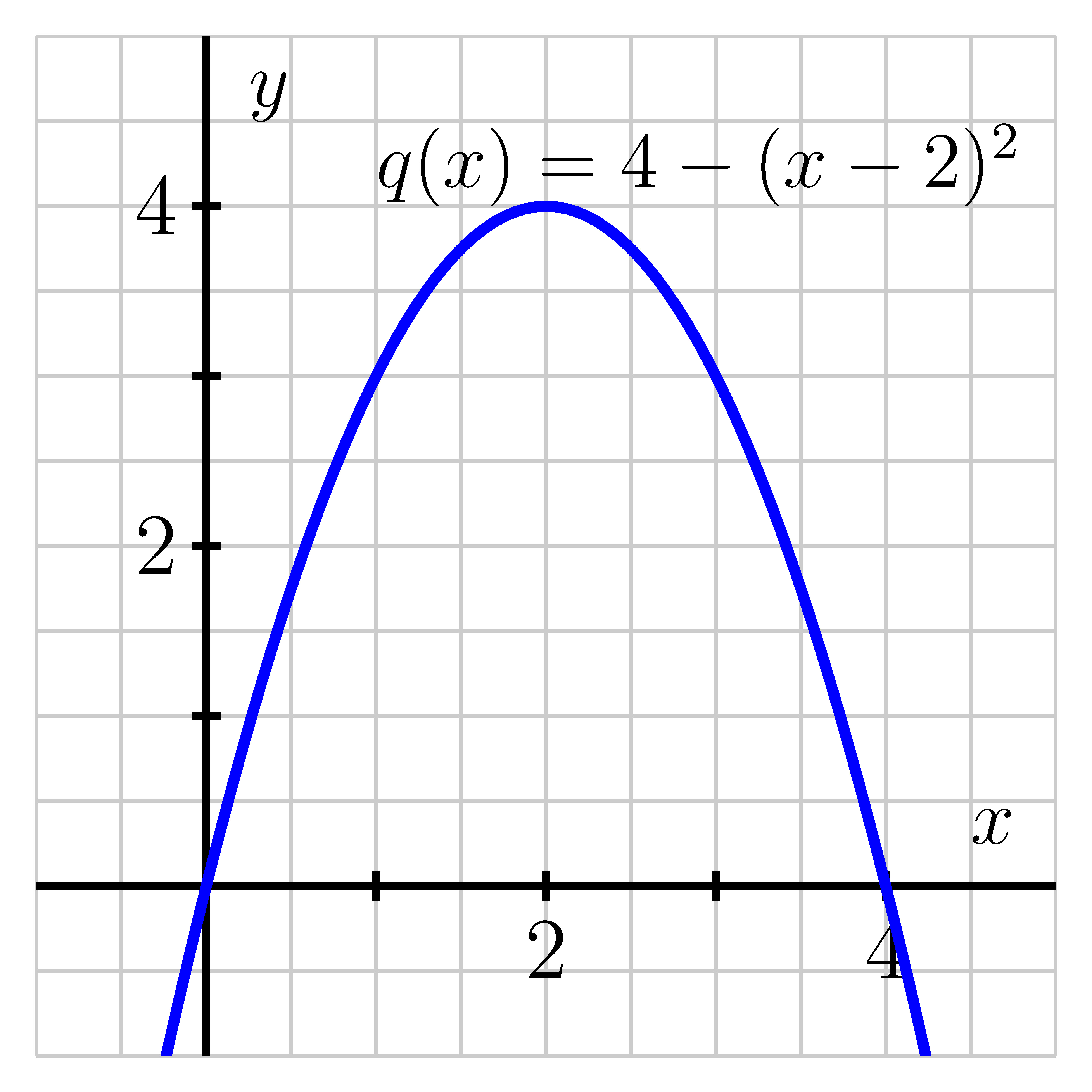
Let’s consider two different functions and see how different computations of their
average rate of change tells us about their respective behavior. Plots of and are
shown below.
- a.
- Consider the function . Compute , , , and . What do your last two computations tell you about the behavior of the function on ?
- b.
- Consider the function . Compute , , and . What do your computations tell you about the behavior of the function on ?
- c.
- On the graphs below, plot the line segments whose respective slopes are
the average rates of change you computed in (a) and (b).
- d.
- True or false: Since , the function is increasing on the interval . Justify your decision.
- e.
- Give an example of a function that has the same average rate of change no matter what interval you choose. You can provide your example through a table, a graph, or a formula; regardless of your choice, write a sentence to explain.
It is helpful be able to connect information about a function’s average rate of change and its graph. For instance, if we have determined that for some function , this tells us that, on average, the function rises between the points and and does so at an average rate of vertical units for every horizontal unit. Moreover, we can even determine that the difference between and is
since . Sketch at least two different possible graphs that satisfy the criteria for the
function stated in each part. Make your graphs as significantly different
as you can. If it is impossible for a graph to satisfy the criteria, explain
why.
- a.
- is a function defined on such that and .
- b.
- is a function defined on such that , , and is not always increasing on
.
- c.
- is a function defined on such that , and .
- For a function defined on an interval , the average rate of change of on is the quantity
- The value of tells us how much the function rises or falls, on average, for each additional unit we move to the right on the graph. For instance, if , this means that for additional -unit increase in the value of on the interval , the function increases, on average, by units. In applied settings, the units of are “units of output per unit of input”.
- The value of is also the slope of the line that passes through the points and
on the graph of , as shown in the graph below.

- This line passing through these two points and , is called a secant line to the graph, and its slope is equal to the average rate of change of the function on the interval .