Accessibility statement: A WCAG2.1AA compliant version of these notes will eventually be available, once I finish writing them. You can also download the TeX source file.
1 About this webpage
These lecture notes were created with Ximera, an interactive textbook platform hosted by Ohio State University. The Ximera Project is funded 2024-2026 (with no other external funding) by a $2,125,000 Open Textbooks Pilot Program grant from the federal Department of Education.
These notes have not yet been peer–reviewed. To load the most updated version, click the orange “update” button at the top of the page. If it is not there, then you are reading the most up-to-date version. The button looks like this:

Funding was provided by The London Mathematical Society and Lancaster University, University of Bristol, University of Edinburgh, Warwick University, Queen Mary University of London, and Ximera.
2 Introductory example
While this appendix does depend on the main document, I will also try to make this as self–contained as possible. To that end, I will provide a well-known motivation coming from quantum harmonic oscillators. Even from this most basic example, we will be able to conclude that orthogonal polynomials occur in the matrix entries of representations. Since vertex weights are entries of the \(R\)–matrix coming from representation theory, we expect that vertex weights are orthogonal polynomials.
In contrast to classical mechanics where position and momentum are either vectors or scalars, in quantum mechanics these are operators. In general, these operators do not commute, and the non–commutativity of the position and momentum operators is related to Heisenberg’s uncertainty principle. If the two operators commuted, then both position and momentum could be measured simultaneously. Furthermore, states in a quantum mechanical system are actually “wavefunctions,” which are modeled as an element of some Hilbert space (on which the operators act).
In one dimension, for example, the position operator \(\hat {x}\) is multiplication by \(x\) while the momentum operator \( \hat {p}\) is \(-i \hbar \frac {\partial }{\partial x}. \) One can verify that if \( f_n \) denotes the function \(x^n\) then \[ \hat {x}\hat {p} f_n = - i \hbar n f_n , \quad \hat {p}\hat {x} = -i \hbar (n+1)f_n, \] and so (using Lie bracket notation) \[ [\hat {p}, \hat {x}]f_n = - i \hbar f_n \neq 0. \]
More generally, the time–dependent Schrödinger’s equation states that for the Hamiltonian operator \(\hat {H}\) and a time–dependent state \( \Psi (t) \) we have \[ i\hbar \frac {d}{dt} \vert \Psi (t) \rangle = \hat {H} \vert \Psi (t) \rangle \] where \(i\) is the imaginary unit and \(\hbar \) is Planck’s constant. In the time–independent version, we consider the case when \( \Psi (t) \) is a stationary state, so \( \Psi (t) = \Psi \) for all times \(t\). Then Schrödinger’s equation tells us that \[ \hat {H} \vert \Psi \rangle = E \vert \Psi \rangle , \] where \(E\) is the energy of the state. Note that this means that the energy can only take discrete, “quantized” values. Generally speaking, the Hamiltonian can be expressed as \[ \hat {H} = \hat {T} + \hat {V} \] where \(\hat {T} \) and \( \hat {V} \) are the kinetic and potential energy.
2.1 Quantum Harmonic Oscillator and Hermite Polynomials
For the harmonic oscillator, we get (in analogy with the classical harmonic oscillator) \[ \frac {\hat {p}^2}{2m} + \frac {1}{2}k \hat {x}^2. \] Plugging in \( \hat {p},\hat {x} \) we get a differential equation which can be explicitly solved. More specifically, the steady states are \[ \psi _n(x) = \frac {1}{\sqrt {2^n\,n!}} \left (\frac {m\omega }{\pi \hbar }\right )^{1/4} e^{- \frac {m\omega x^2}{2 \hbar }} H_n\left (\sqrt {\frac {m\omega }{\hbar }} x \right ), \qquad n = 0,1,2,\ldots . \] where \(H_n\) are the physicists’ Hermite polynomials \[ H_n(z)=(-1)^n e^{z^2}\frac {d^n}{dz^n}\left (e^{-z^2}\right ). \] The corresponding energy levels are: \[ E_n = \hbar \omega \bigl (n + \tfrac {1}{2}\bigr ). \] The Hermite polynomials are orthogonal polynomials in the sense that \[ \int _{-\infty }^{\infty } H_m(x) H_n(x) e^{-x^2}dx = \sqrt {\pi }2^n n! \delta _{nm}. \] They satisfy the generating function \[ e^{2xt - t^2} = \sum _{n=0}^\infty H_n(x) \frac {t^n}{n!} \] and the recurrence relation \[ H_{n+1}(x) = 2xH_n(x) - 2nH_{n-1}(x). \]
2.2 CCR relations and Lie algebras
Now, what does this have to do with Lie algebras? To answer this, we approach the quantum harmonic oscillator using “ladder operators.” Define two abstract algebra elements \( \hat {a} \text { and }\hat {a}^{\dagger }\) with canonical commutation relation \[ [\hat {a}, \hat {a}^{\dagger }]=1. \] There is a representation onto an infinite–dimensional vector space with bases \( \vert n \rangle , n=0,1,2\) given by \[ \begin{align} \hat {a}^\dagger |n\rangle &= \sqrt {n + 1} | n + 1\rangle \\ \hat {a}|n\rangle &= \sqrt {n} | n - 1\rangle . \end{align} \] For this reason, \(\hat {a}\) and \(\hat {a}^{\dagger }\) are called lowering and raising operators, respectively. We also introduce a “number operator” \[ \begin{align} N &= \hat {a}^\dagger \hat {a} \\ N\left | n \right \rangle &= n\left | n \right \rangle . \end{align} \]
In the context of the quantum harmonic oscillator, these algebra elements can be represented as \begin{align} \hat {a} &=\sqrt {m\omega \over 2\hbar } \left (\hat x + {i \over m \omega } \hat p \right ), \\ \hat {a}^\dagger &=\sqrt {m\omega \over 2\hbar } \left (\hat x - {i \over m \omega } \hat p \right ). \end{align}
Then \[ \hat {H} = \hbar \omega \left (N + \frac {1}{2}\right ), \] so the energy levels are \(E_n = n + \tfrac {1}{2},\) as we found before.
To relate the two methods in more mathematical formalism, we define the Hilbert space \(L^2(\mathbb {R},w) \) of square–integrable functions on \(\mathbb {R}\) with respect to the weight \(w(x)=e^{-x^2/2}.\) Then this Hilbert space has an orthogonal basis \( \{H_n: n \geq 0\} \) consisting of the Hermite polynomials. If we let \(\mathcal {A}\) denote the algebra generated by \(\hat {a},\hat {a}^{\dagger }\) then we just defined a representation of \(\mathcal {A}\) on \(L^2(\mathbb {R},w)\) where \(\vert n \rangle = H_n. \) Note that we can define a map from \(\mathcal {A}\) to \(B(L^2(\mathbb {R},w))\). Using the generating function and recurrence relation, we have \[ x H_n(x) = \frac {1}{2}H_{n+1}(x) + n H_{n-1}(x) \] and \[ \frac {d}{dx} H_n(x) = 2n H_{n-1}(x). \] Then the ladder operators act as \[ \hat {a} = \frac {1}{\sqrt {2}}\left (x + \frac {d}{dx}\right ), \quad \hat {a}^\dagger = \frac {1}{\sqrt {2}}\left (x - \frac {d}{dx}\right ). \] Then using the formulas above, these act on the wavefunctions as \[ \hat {a}^\dagger \psi _n = \sqrt {n+1} \, \psi _{n+1} \] \[ \hat {a} \psi _n = \sqrt {n} \, \psi _{n-1} \]
Next, we relate Lie algebras to ladder operators using the Jordan–Schwinger realization. It may be more illustrative to demonstrate this first in the case of \(\mathfrak {sl}_2\). Let \(\mathcal {A}_n\) be generated by \(\hat {a}_i,\hat {a}_i^{\dagger }, i=1,2,\ldots ,n\) with the commutation relations \[ [\hat {a}_i, \hat {a}_j^{\dagger }]=1 \delta _{ij}, \quad [\hat {a}_i,\hat {a}_j] = [\hat {a}^{\dagger }_i, \hat {a}^{\dagger }_j]=0 \text { for } i\neq j. \] The Jordan–Schwinger realization of \(\mathfrak {sl}_2\) is then an injection from \(\mathfrak {sl}_2\) to \(\mathcal {A}_2\). In a typical physics introduction, this example is discussed in the context of angular momentum. In this context, we recall the Pauli spin matrices \[ \sigma ^1 = \left (\begin{array}{cc} 0 & 1 \\ 1 & 0 \end{array}\right ), \quad \quad \sigma ^2 = \left ( \begin{array}{cc} 0 & -i \\ i & 0 \end{array}\right ), \quad \quad \sigma ^3 = \left ( \begin{array}{cc} 1 & 0 \\ 0 & -1 \end{array}\right ). \] which span \(\mathfrak {sl_2}\). The change of basis to \(e,f,h\) is given by \begin{align*} e &= \frac {\sigma _1 + i\sigma _2}{2} & \sigma _1 &= e+f \\ f &= \frac {\sigma _1 - i\sigma _2}{2} & \sigma _2 &= -i(e-f) \\ h &= \sigma _3 & \sigma _3 &= h \end{align*}
The Pauli matrices are then written in terms of the ladder operators as \[ \sigma _1 = \hat {a}_1\hat {a}_2^{\dagger } + \hat {a}_1^{\dagger }\hat {a}_2, \quad \sigma _2 = -i( \hat {a}_1^{\dagger }\hat {a}_2 - \hat {a}_1\hat {a}_2^{\dagger } ), \quad \sigma _3 = \hat {a}_1^{\dagger }\hat {a}_1 - \hat {a}_2^{\dagger }\hat {a}_2 \] By comparing the last formula to the change of basis, it is reasonable to conjecture that the elements \(\hat {a}_1^{\dagger }\hat {a}_2, \hat {a}_1\hat {a}_2^{\dagger }, \hat {a}_1^{\dagger }\hat {a}_1 - \hat {a}_2^{\dagger }\hat {a}_2\) then satisfy the same relations as \(e,f,h\in \mathfrak {sl}_2\), respectively. Indeed this is the case; for example, the relation \([h,e]=2e\) can be seen in \begin{align*} \left ( \hat {a}_1^{\dagger }\hat {a}_1 - \hat {a}_2^{\dagger }\hat {a}_2 \right ) \cdot \left ( \hat {a}_1^{\dagger }\hat {a}_2 \right ) &= \hat {a}_1^{\dagger }\hat {a}_1\hat {a}_1^{\dagger }\hat {a}_2 - \hat {a}_2^{\dagger }\hat {a}_2\hat {a}_1^{\dagger }\hat {a}_2\\ &= \hat {a}_1^{\dagger }( \hat {a}_1^{\dagger }\hat {a}_1 + 1)\hat {a}_2 - \hat {a}_1^{\dagger } (\hat {a}_2\hat {a}_2^{\dagger } - 1) \hat {a}_2 \\ &= \hat {a}_1^{\dagger }\hat {a}_2\hat {a}_1^{\dagger }\hat {a}_1 + \hat {a}_1^{\dagger }\hat {a}_2 - \hat {a}_1^{\dagger }\hat {a}_2\hat {a}_2^{\dagger }\hat {a}_2 + \hat {a}_1^{\dagger }\hat {a}_2 \\ &= \left ( \hat {a}_1^{\dagger }\hat {a}_2 \right )\cdot \left ( \hat {a}_1^{\dagger }\hat {a}_1 - \hat {a}_2^{\dagger }\hat {a}_2 +2\right ). \end{align*}
More generally, there is an injection from any finite–dimensional Lie algbra \(\mathfrak {g}\) to some \(\mathcal {A}_n\). Since there is an injection \(\mathrm {ad}: \mathfrak {g} \rightarrow \mathfrak {gl}(\mathfrak {g})\), without loss of generality we can take \( \mathfrak {g} = \mathfrak {gl}(n)\). The Jordan–Schwinger realization is then an injection of Lie algebras defined by \[ M \rightarrow \sum _{i,j=1}^n \hat {a}^{\dagger }_i M_{ij} \hat {a}_j. \] One can check that this generalizes the case when \(\mathfrak {g}=\mathfrak {sl}_2\).
As a result, if there is a Jordan–Schwinger realization \(\mathfrak {g} \hookrightarrow \mathcal {A}_n\) then any representation of \(\mathcal {A}_n\) pulls back to a representation of \(\mathfrak {g}.\) Since we have already seen the Hermite polynomials appear as an orthonormal basis of a representation of \(\mathcal {A}_1\), it is not unreasonable to expect orthogonal polynomials to appear in the representations of \(\mathfrak {g}.\) Note that if we had instead picked a basis of \(1,x,x^2,\ldots \), then after a change of basis, we would see the Hermite polynomials in the matrix elements of representations of \(\mathcal {A}_1\).
Of course, the Jordan–Schwinger realization does not produce interesting examples of Lie algebras inside \(\mathcal {A}_1\), so we will have to go to higher–dimensional examples. This will result in generalizations of the Hermite polynomials, which leads into the next section.
3 Hierarchy of Orthogonal Polynomials
The Askey–Wilson scheme is a way of organizing orthogonal polynomials of hypergeometric or basic hypergeometric type into a hierarchy. Below is the hierarchy for basic hypergeometric type (courtesy of Koornwinder):
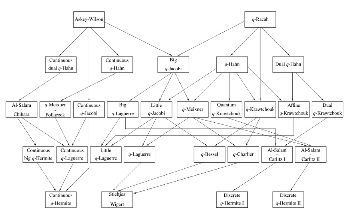
Note that Hermite polynomials are in this flowchart, as a \(q\rightarrow 1\) limit of the various \(q\)–Hermite polynomials. We note that the \(q\)–deformation here is a different quantization than the quantization in the quantum harmonic oscillator; roughly, this corresponds to quantizing the product in one case, and quantizing the co–product in the other case.
3.1 Definitions
Define the \(q\)–Pochhammer symbol by \[ (a;q)_n = (1-a)(1-aq) \cdots (1-aq^{n-1}) \] and \[ (a_1,\ldots ,a_r)_n = (a_1;q)_n \cdots (a_r;q)_n \] The basic hypergeometric series, or \(q\)–hypergeometric series is defined by ([KLSBook]) \[ { }_{r} \phi _{s}\left [\begin{array}{cccc}a_{1} & a_{2} & \ldots & a_{j} \\ b_{1} & b_{2} & \ldots & b_{k}\end{array} ; q, z\right ] :=\sum _{k=0}^{\infty } \frac {\left (a_{1}, \ldots , a_{r} ; q\right )_{k}}{\left (b_{1}, \ldots , b_{s} ; q\right )_{k}}(-1)^{(1+s-r) k} q^{(1+s-r)\binom {k}{2}} \frac {z^{k}}{(q ; q)_{k}} \] The various orthogonal polynomials are defined in terms of the \(q\)–hypergeometric series. Note that if \(a_1=q^{-n}\) then the series terminates, justifiably calling it a polynomial. One example are \(q\)–Racah polynomials, which are defined by \[ R_{n}(\mu (x) ; \alpha , \beta , \gamma , \delta | q) = { }_{4} \phi _{3}\left (\begin{array}{c}q^{-n}, \alpha \beta q^{n+1}, q^{-x}, \gamma \delta q^{x+1} \\ \alpha q, \beta \delta q, \gamma q\end{array} ; q, q\right ), n = 0,1,2,\ldots , N. \] where \[ \mu (x):=q^{-x}+\gamma \delta q^{x+1} \] and \[ \alpha q=q^{-N} \quad \text { or } \quad \beta \delta q=q^{-N} \quad \text { or } \quad \gamma q=q^{-N}. \] Note that \( {}_{4} \phi _{3} \) depends on seven variables whereas the \(q\)–Racah depends on six variables; if the relation \(a_1a_2a_3a_4 = q^{-1}b_1b_2b_3\) holds, and one of \( \{b_1,b_2,b_3\}\) is of the form \(q^{-N}\), then the \( {}_4 \phi _{3} \) function can be written as a \(q\)–Racah.
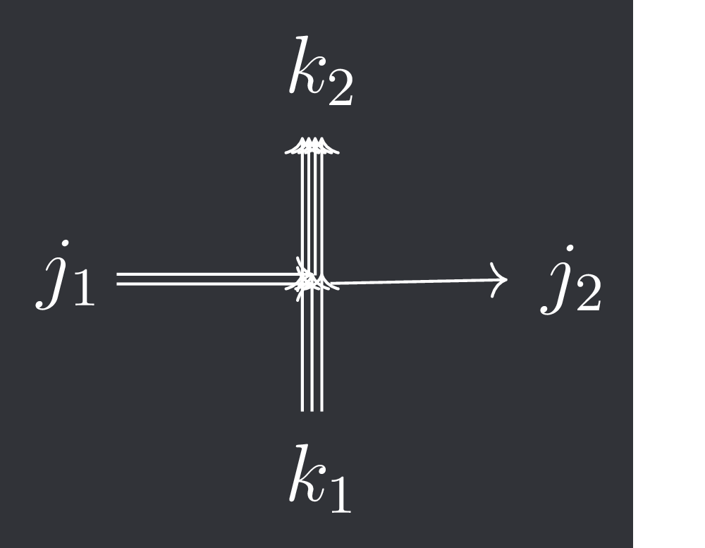
It turns out that the weights of the \(R\)–matrix of \( \mathcal {U}_q(\widehat {sl_2}) \) are given by the \(q\)–Racah polynomials. Before stating that result, we define some notation. We will let \(m\) denote the maximum number of particles that can enter from the vertical direction, and let \(l\) denote the maximum number of particles that can enter from the horizontal direction. So the stochastic matrix is an operator on \(V_l \otimes V_m\) where \(V_l\) is \(l+1\)–dimensional and \(V_m\) is \(m+1\)–dimensional. We denote a matrix entry by \[ [S(z)]_{j_1,k_1}^{j_2,k_2}, \quad 1 \leq j_1,j_2 \leq l, \quad 1 \leq k_1,k_2 \leq m. \] This corresponds to this weight:
Of course, the weights of the \(R\)–matrix are generally not stochastic. There is a type of transformation that will make it stochastic.
We will state a theorem from [CP16] and [Kua18]; see also [KMMO16] and [BM16] for higher rank generalizations; and the previous papers of [Pov13] and [Man14].
Note that the reason I used \(\nu =q^{-m}\) is that the value \(\nu \) can be extended to arbitrary complex numbers through analytic continuation. I believe this can be done algebraically through Verma modules, but I’m not sure.
The proof of this theorem is essentially in two parts. In Theorem 3.15 of [CP16], the authors prove that applying Rogers–Pitman intertwining results in stochastic vertex weights expressed in terms of the \(q\)–Racah polynomials. In [Kua18], I prove that applying Rogers–Pitman intertwining “commutes” with the gauge transformation, in the sense that first applying the gauge transformation and then applying fusion results in the same matrix as first applying fusion and then applying the gauge transformation. Thus, the stochastic matrix \(S\) has the necessary algebraic properties to prove Markov duality.
I’ll only sketch the argument. The proof that Rogers–Pitman intertwining “commutes” with the gauge transformation is in Theorem 3.4 of [Kua18], and is a long calculation that is not particularly enlightening. The proof that the \(q\)–Racah polynomials occur is due to a recurrence relation that comes from fusion. Before that, we consider the \(l=1\) case, so that the weights appear in Figure 1.
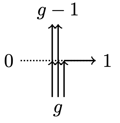
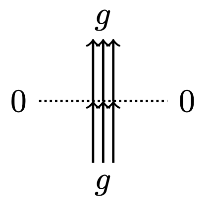
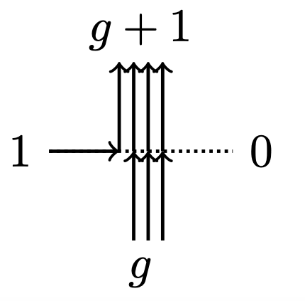
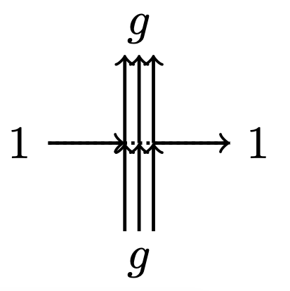
Those weights are simple enough to calculate. Next, we fuse in the vertical direction. Figure 2 below shows the intuition for the argument. If \(j_1\) arrows come in from the left, where at most \(l\) arrows are allowed, we choose random places for the arrows across two vertices where at most \(l-1\) and \(1\) arrows are allowed. The random placement has a nice combinatorial description. Define the \(q\)–deformed integer, factorial and binomial by \[ [n]_q = \frac {1-q^n}{1-q}, \quad [n]_q^! = [1]_q \cdots [n]_q, \quad \binom {l}{j}_q = \frac {[l]_q^!}{[j]_q^! [l-j]_q^!}. \] Then we have the relation \[ \binom {l}{j}_q = q^j \binom {l-1}{j}_q + \binom {l-1}{j-1}_q. \] So then \[ \mathbf {P}(0)= \frac {q^j\binom {l-1}{j}_q}{\binom {l}{j}_q}, \quad \mathbf {P}(1) = \frac {\binom {l-1}{j-1}_q}{\binom {l}{j}_q}, \] which simplifies to the same probability in Lemma 3.13 of [CP16].
![[Picture]](Orth_Poly-7615502c7616bba59ff87b80fa0ffd21.svg)
In this way, you obtain a recurrence relation in the parameter \(l\). Lemma 3.13 of [CP16] shows that the \(q\)–Racah formula satisfies the same recurrence relation.
References
[BM16] Gary Bosnjak, Vladimir V. Mangazeev, Construction of R-matrices for symmetric tensor representations related to \(U_q(\widehat {sl_n})\). J. Phys. A: Math. Theor. 49 (2016) 495204
[CP16] Corwin, I., Petrov, L. Stochastic Higher Spin Vertex Models on the Line. Commun. Math. Phys. 343, 651–700 (2016).
[KLSBook] Roelof Koekoek , Peter A. Lesky , René F. Swarttouw, Hypergeometric Orthogonal Polynomials and Their q-Analogues, Springer 2010.
[Kua18] J. Kuan, An algebraic construction of duality functions for the stochastic \( U_q(A_n^{(1)}) \) vertex model and its degenerations, Commun. Math. Phys. (2018) 359: 121
[KMMO16] A. Kuniba, V.V. Mangazeev, S. Maruyama, M. Okado, Stochastic R matrix for \(U_q(A_n^{(1)})\), Nuclear Physics B, Volume 913, 2016, Pages 248-277.
[Man14] Vladimir V. Mangazeev, On the Yang–Baxter equation for the six-vertex model, Nuclear Physics B, Volume 882, May 2014, Pages 70-96
[Pov13] A.M. Povolotsky, On the integrability of zero-range chipping models with factorized steady states J. Phys. A, Math. Theor., 46 (2013), p. 465205